1. Project Overview
Background and Goals
As the final project for a reinforcement learning course, I implemented three algorithms myself, DQN (Deep Q-Network), Double DQN, and PER (Prioritized Experience Replay), and compared their performance. Rather than just using a library, the goal was to implement the core algorithms from scratch in PyTorch and gain a deep understanding of how each one works and what characterizes it.
In particular, I wanted to answer three questions:
- How much does DQN's Q-value overestimation problem actually affect performance?
- Does Double DQN outperform DQN in every environment?
- Can PER solve the fundamental problem of sparse-reward environments?
I tested the implemented algorithms in three OpenAI Gymnasium environments, CartPole-v1, Acrobot-v1, and MountainCar-v0, to identify the characteristics and limits of each algorithm. The three environments each have a different reward structure and difficulty, which makes them well suited for comparing algorithms.
Reinforcement Learning Basics
Before getting into the algorithms, I summarized the core concepts of reinforcement learning.
Markov Decision Process (MDP)
A reinforcement learning problem is formalized as a Markov Decision Process (MDP). An MDP consists of the following elements:
- State space S: the set of all states the agent can be in
- Action space A: the set of all actions the agent can take
- Transition probability P(s'|s,a): the probability of moving to state s' after taking action a in state s
- Reward function R(s,a,s'): the immediate reward for a transition
- Discount factor γ: the rate at which future rewards are discounted to present value (0 ≤ γ ≤ 1)
The agent's goal is to find a policy π that maximizes the expected cumulative reward.
The Q-Function and the Bellman Equation
The Q-function Q(s,a) represents the expected cumulative reward obtained by taking action a in state s and then following policy π. The optimal Q-function satisfies the Bellman optimality equation:
Q-Learning learns the optimal Q-function by applying this equation repeatedly. Tabular Q-Learning works well when the number of state-action pairs is small, but continuous or high-dimensional state spaces require function approximation.
The Rise of Deep Reinforcement Learning
In 2013, DeepMind proposed DQN, which approximates the Q-function with a neural network. But simply using a neural network made training unstable. Two key techniques solved this problem:
- Experience Replay: store experiences in a buffer and sample them randomly to break the correlation between data points
- Target Network: use a separate target network to keep the learning target stable
These two techniques became the foundation for later algorithms such as Double DQN and PER.
Experimental Environments
The three environments used in this project each have different characteristics, which makes them well suited for comparing algorithms.
CartPole-v1
An environment where you move a cart with a pole attached left and right to keep the pole balanced. Keeping the pole up for 500 steps counts as success.
- State space: cart position, cart velocity, pole angle, pole angular velocity (4-dimensional, continuous)
- Action space: left/right (2, discrete)
- Reward: +1 every step (dense reward)
- Termination: pole angle beyond ±12°, cart position beyond ±2.4, or 500 steps reached
CartPole is called the "Hello World" of reinforcement learning and is widely used to test algorithms. Its 4-dimensional state space is relatively simple, and the +1 reward every step makes the learning signal dense. Keeping the balance looks intuitively easy, but even a slightly wrong policy fails quickly, which makes it good for testing policy stability.
Acrobot-v1
An environment where you swing a pendulum made of two linked segments to raise its tip to a target height. It has complex pendulum dynamics.
- State space: cos/sin of the two links and their angular velocities (6-dimensional, continuous)
- Action space: torque -1, 0, +1 (3, discrete)
- Reward: -1 every step until the goal is reached (dense negative reward)
- Termination: tip reaches the target height, or more than 500 steps
With its 6-dimensional state space, Acrobot looks more complex than CartPole, but the -1 reward every step gives a clear learning signal: "reach the goal fast." It has to learn a complex swinging motion, but thanks to the dense reward structure, training is relatively stable.
MountainCar-v0
An environment where you accelerate a car in a valley left and right to reach the top of the hill on the right. It is a textbook example of the sparse reward problem.
- State space: position, velocity (2-dimensional, continuous)
- Action space: accelerate left, do nothing, accelerate right (3, discrete)
- Reward: 0 only when the goal is reached, -1 otherwise (sparse reward)
- Termination: position reaches 0.5 or more, or more than 200 steps
MountainCar has the simplest state space, at 2 dimensions, but its sparse reward structure makes it the hardest. The car's engine is too weak to beat gravity, so it cannot drive straight up the hill and has to build momentum on the opposite slope. Until it discovers this "swing" strategy, it cannot reach the goal and gets no meaningful learning signal. It is the classic environment for showing the importance of exploration.
Development Environment
- Framework: PyTorch 2.0
- Environment library: OpenAI Gymnasium 0.29
- Hardware: NVIDIA RTX 3080 GPU
- Experiment runs: 1000 epochs per algorithm-environment combination
2. Network Architecture Design
I designed all three algorithms to use the same Q-Network architecture. This makes it possible to isolate the effect of the algorithms themselves on performance, rather than differences in network architecture.
Q-Network Implementation
The architecture has two hidden layers (128 units) with ReLU activation. The input is the state vector, and the output is the Q-value of each action.
Design Decisions
Choosing the Hidden Layer Size
The reasons for setting the hidden layer size to 128:
- The state spaces of the experimental environments are relatively small, at 2~6 dimensions
- 128 units strike a balance between expressive power and computational efficiency
- A larger network risks overfitting, and a smaller one risks lacking expressive power
In early experiments testing 64, 128, and 256 units, 128 units gave stable performance in all three environments.
Choosing the Activation Function
Why ReLU:
- Computationally efficient (a simple max operation)
- Mitigates the vanishing gradient problem
- Used in the original DQN paper, which helps reproducibility
Choosing the Loss Function
I used Smooth L1 Loss (Huber Loss). Advantages over MSE Loss:
- Less sensitive to outliers
- Stable in the early training stage, when TD errors are large
- The approach recommended in the original DQN paper
3. DQN Implementation
What Is DQN?
DQN (Deep Q-Network) is an algorithm that applies deep learning to Q-Learning. DeepMind first proposed it in 2013, and its 2015 Nature paper reached human-level performance on Atari games, opening the era of deep reinforcement learning.
Core Idea
Traditional Q-Learning stores the Q-value of every state-action pair in a table. But when the state space is large or continuous, the table approach is impossible. DQN learns Q(s,a; θ) using a neural network as the function approximator.
The Training Instability Problem
Simply using a neural network makes training unstable. There are two causes:
- Data correlation: consecutive states are similar to each other, violating the i.i.d. assumption
- Moving target: when updating Q-values, the target is computed with the same network, making it unstable
DQN's Solutions
-
Experience Replay: store experiences (s, a, r, s', done) in a buffer and sample them randomly. This breaks the correlation between data points and satisfies the i.i.d. condition.
-
Target Network: maintain a separate target network θ⁻. Every fixed interval (e.g., 1000 steps), copy the online network θ into it. This keeps the target stable.
The Q-Value Overestimation Problem
One of DQN's known limitations is Q-value overestimation. When computing the target:
The max operator picks the largest of the noisy Q-value estimates. If the Q-value estimates are noisy, the max operation systematically picks overestimated values. Double DQN solves this problem.
DQN Implementation Details
1) Hyperparameter Settings
I set a different epsilon decay rate for each environment. In particular, since MountainCar is a sparse-reward environment, I applied a slower decay rate to allow enough exploration.
Rationale for the Hyperparameters
- Discount factor 0.98: CartPole's maximum is 500 steps, and γ^500 ≈ 0.00004, so it considers a sufficiently distant future
- Learning rate 0.001: the Adam optimizer's default; stable convergence was confirmed
- Batch size 256: a balance between GPU memory use and lower gradient variance
- Buffer size 100000: ensures enough diversity of experience
2) Action Selection Method (get_action)
I implemented an ε-greedy policy: with probability ε take a random action, and with probability 1-ε take the action with the highest current Q-value.
Heuristic Exploration for MountainCar
In the MountainCar environment, pure random exploration is inefficient. If the car moves randomly at the bottom of the valley, it cannot build momentum and just circles in place. To fix this, I added a heuristic that accelerates in the direction of the velocity:
- If moving right, accelerate right → climb the right hill
- If moving left, accelerate left → build momentum on the left hill
- If stopped, accelerate left or right (standing still is inefficient)
This heuristic naturally induces a swinging motion and raises the chance of reaching the goal.
3) Training Method (train)
I implemented the basic DQN approach that uses in the target computation.
Training Process in Detail
-
Sampling: randomly draw 256 experiences from the buffer. This breaks temporal correlation.
-
Target computation: compute the maximum Q-value of the next state with the target network. Block the gradient with to stabilize the target.
-
TD error: Q(s,a) - target. Minimize the difference between the prediction and the target.
-
Backpropagation: update only the online network. The target network is copied periodically.
4) Target Network Update
At the end of every epoch, the target network was replaced with the online network. I used a hard update. I also tested a soft update (θ⁻ ← τθ + (1-τ)θ⁻), but the performance difference was negligible, so I adopted the hard update for simplicity of implementation.
DQN Results
CartPole-v1 Results
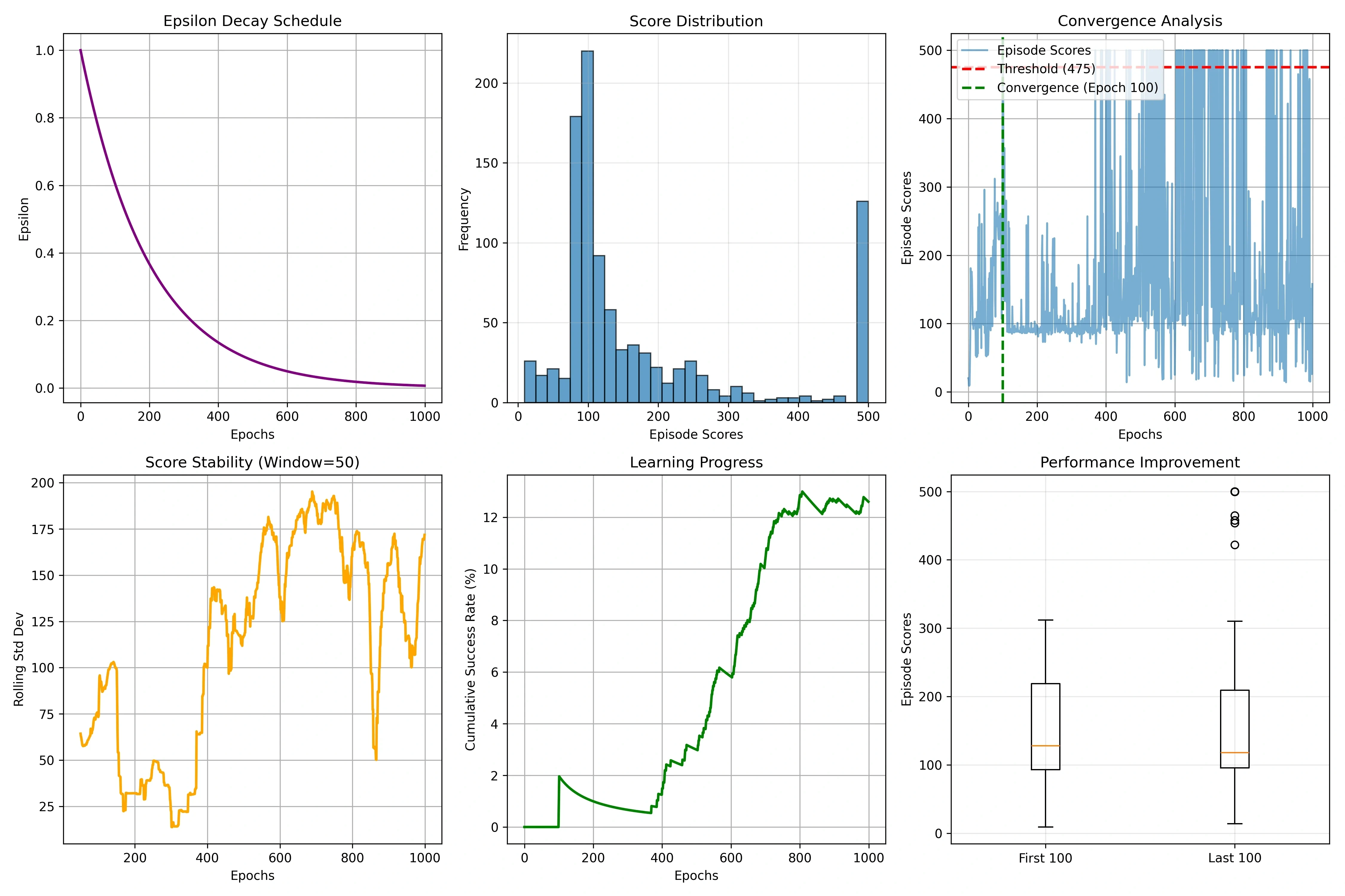
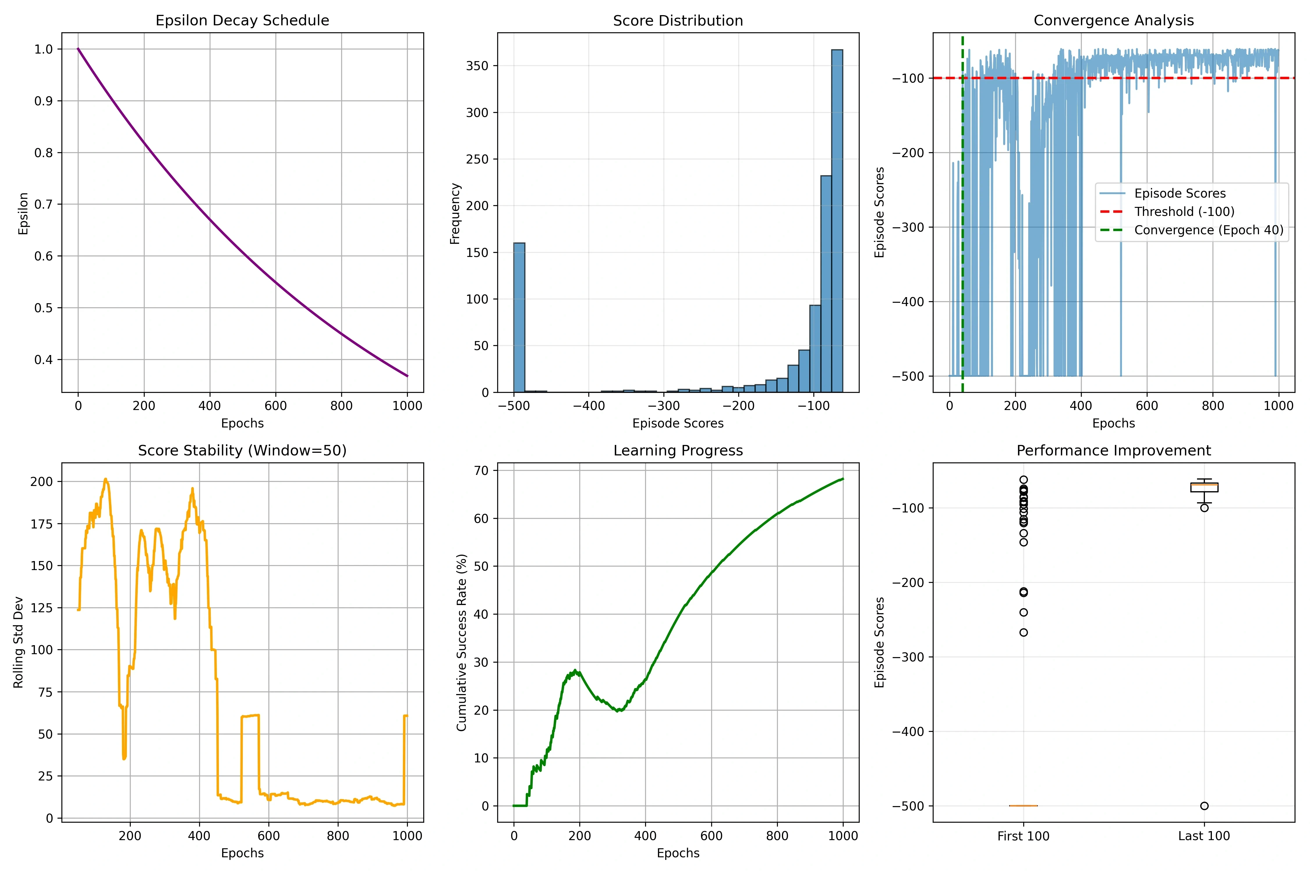
Despite a proper training procedure, DQN showed severe underperformance on CartPole-v1. Figure 1 shows that although epsilon decayed properly from 1.0 to 0.0067, the cumulative success rate stayed at 12%.
The score distribution reveals an interesting pattern. Scores are split into two groups: below 150 (failure) or exactly 500 (perfect success). This indicates "all-or-nothing" behavior, meaning the policy is fragile near the balance point and fails as soon as it becomes unstable. The near absence of intermediate scores (e.g., 300) suggests that the policy does not improve gradually and instead succeeds or fails by luck.
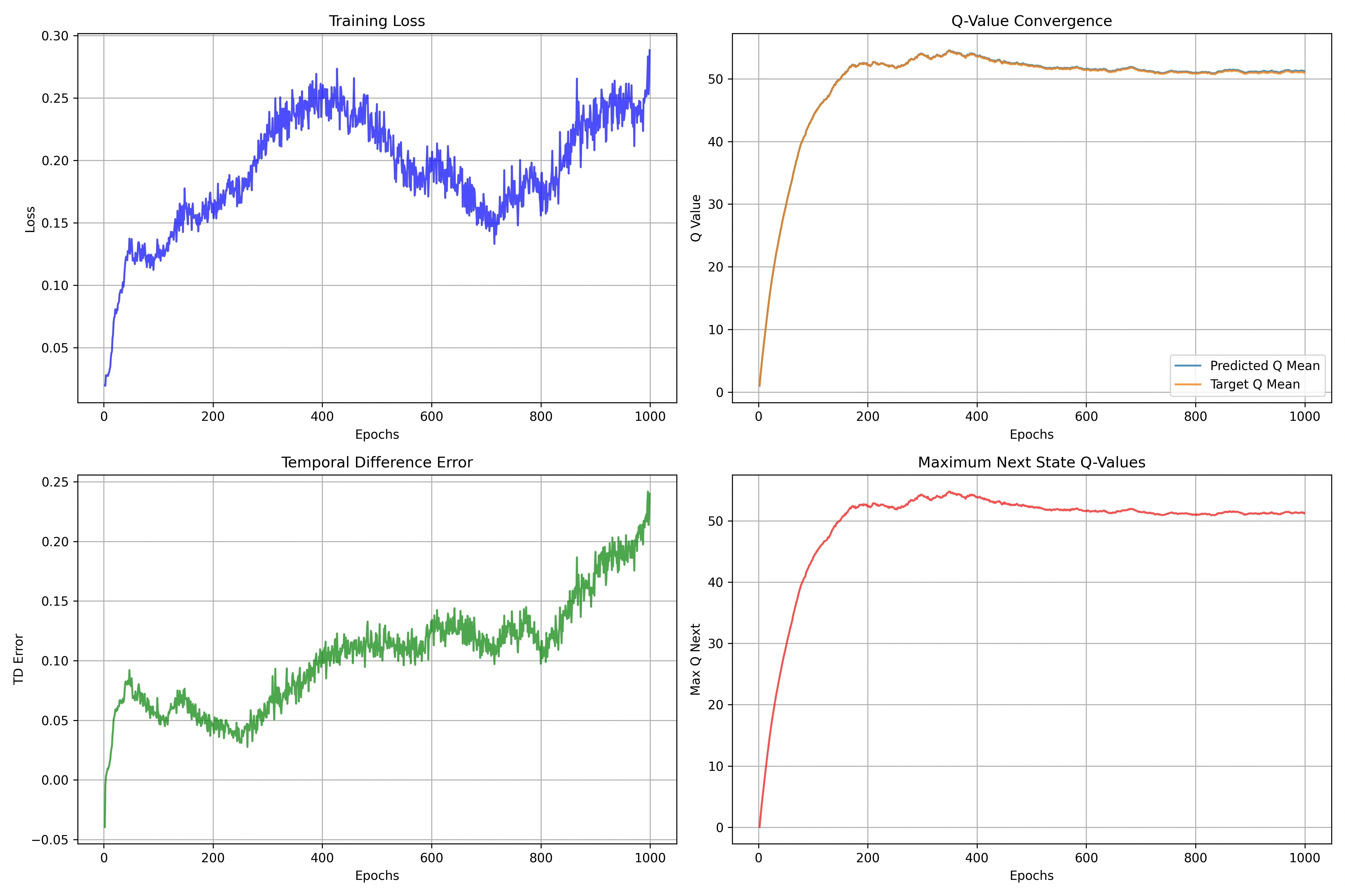
Figure 2 shows the Q-value converging to about 51, which matches the theoretical expectation with γ=0.98. In CartPole the agent receives +1 every step for up to 500 steps, so the theoretical Q-value is:
The Q-value converging to 51 means the value estimate itself is being learned correctly.
However, the TD error rising in later epochs indicates the overestimation bias characteristic of vanilla DQN. As the max operator picks the largest of the noisy Q-values, the Q-values are inflated beyond their true values, and this feeds back into the target, creating a vicious cycle.
The training loss shows non-monotonic behavior with persistent oscillation even after epoch 300. This suggests that the agent has failed to converge to the optimal policy and is stuck in a suboptimal local minimum.
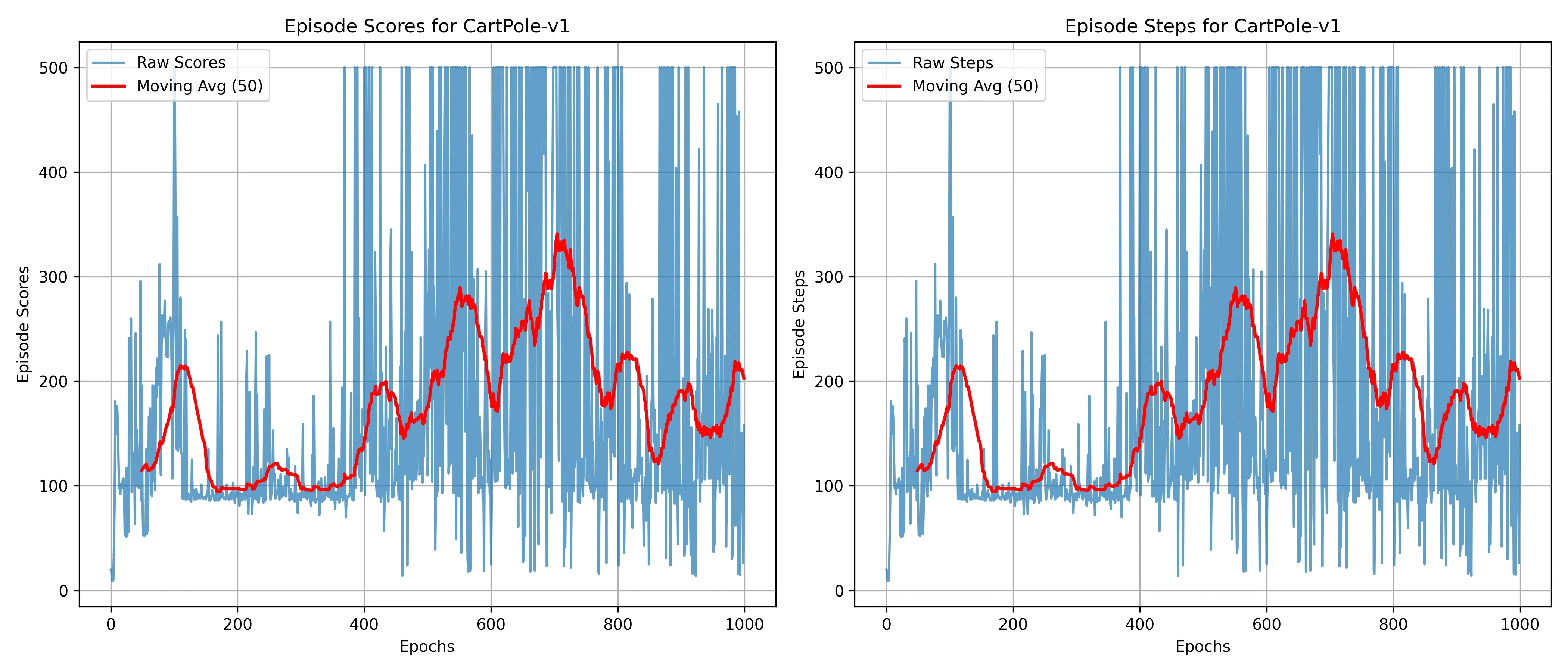
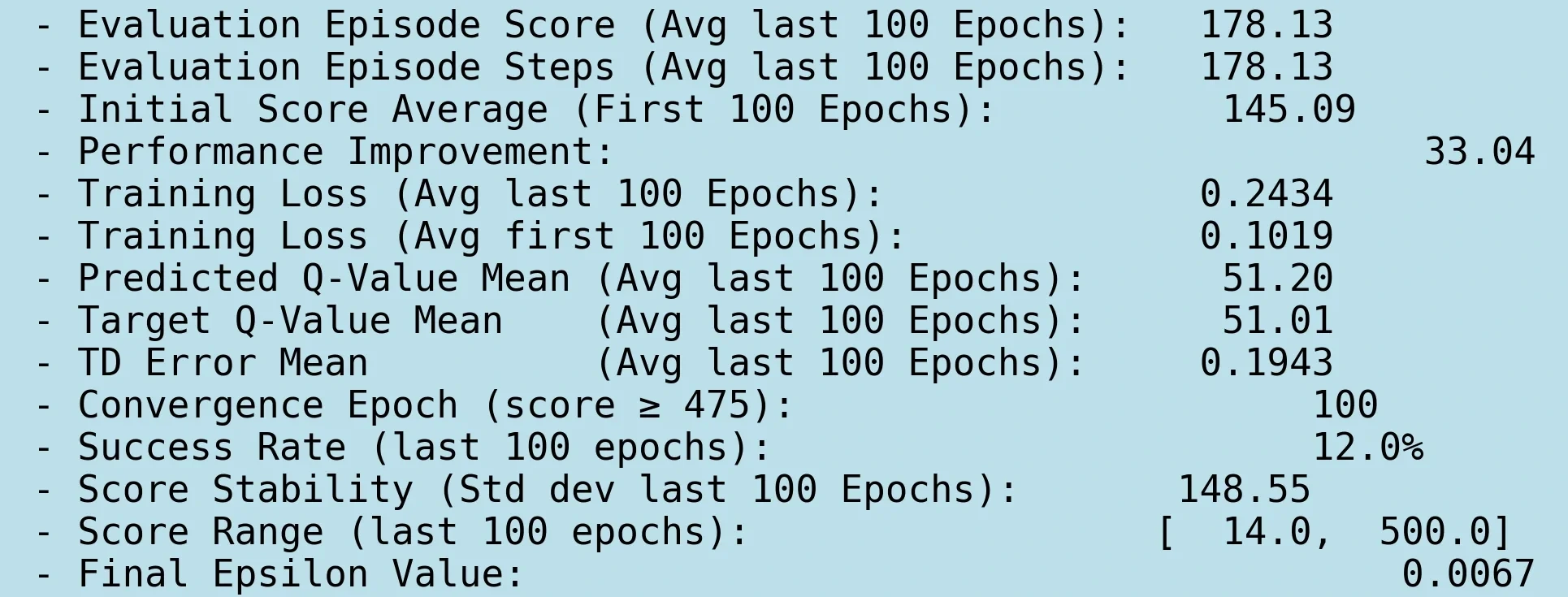
Figure 3 shows persistent score variability even in the final epochs. The agent achieved only 35.6% (178.13/500) of optimal performance. The high variance in Figure 4 (σ=148.55) quantitatively confirms the policy instability. It shows that the agent learned to succeed sporadically but could not maintain consistent performance.
Acrobot-v1 Results
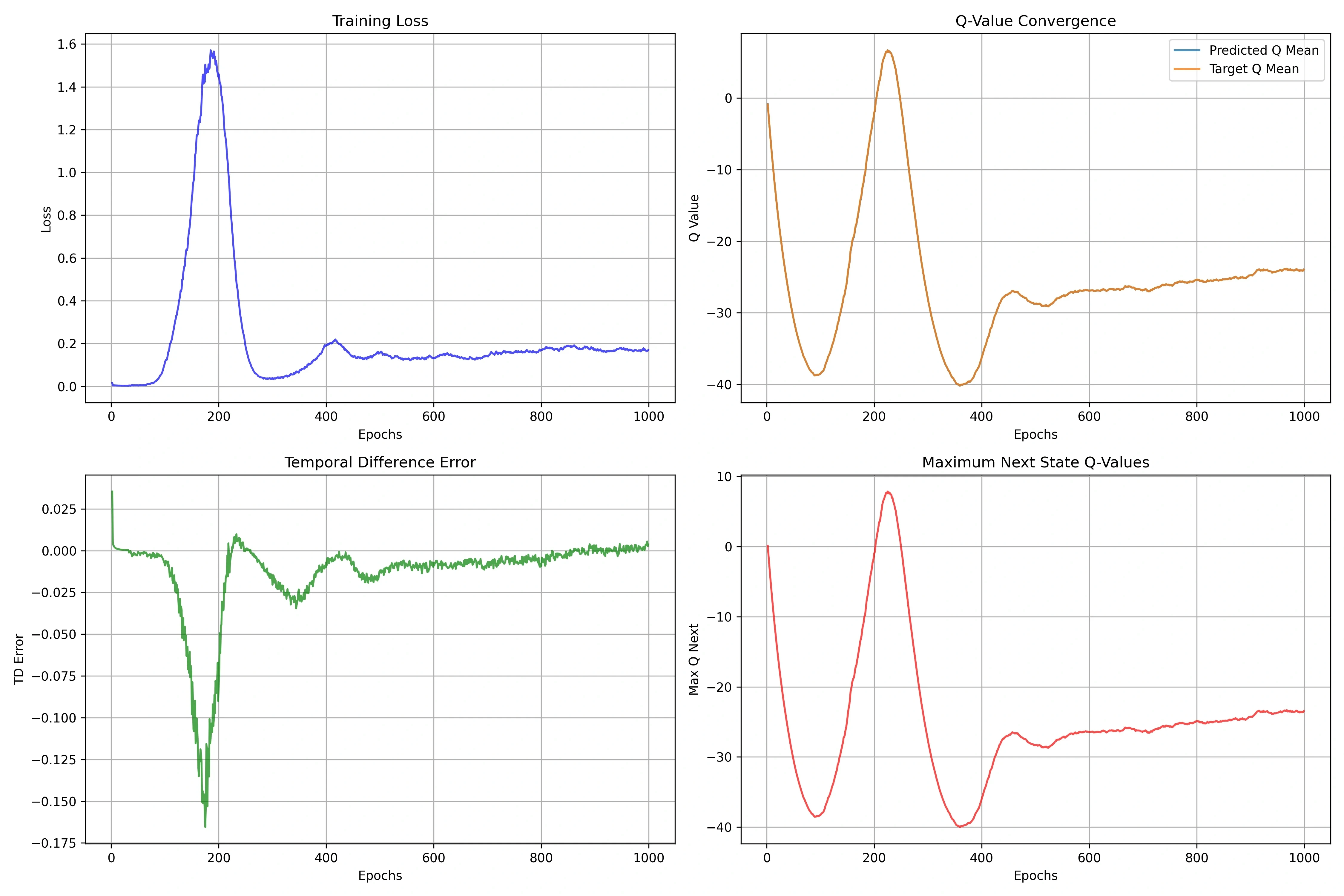
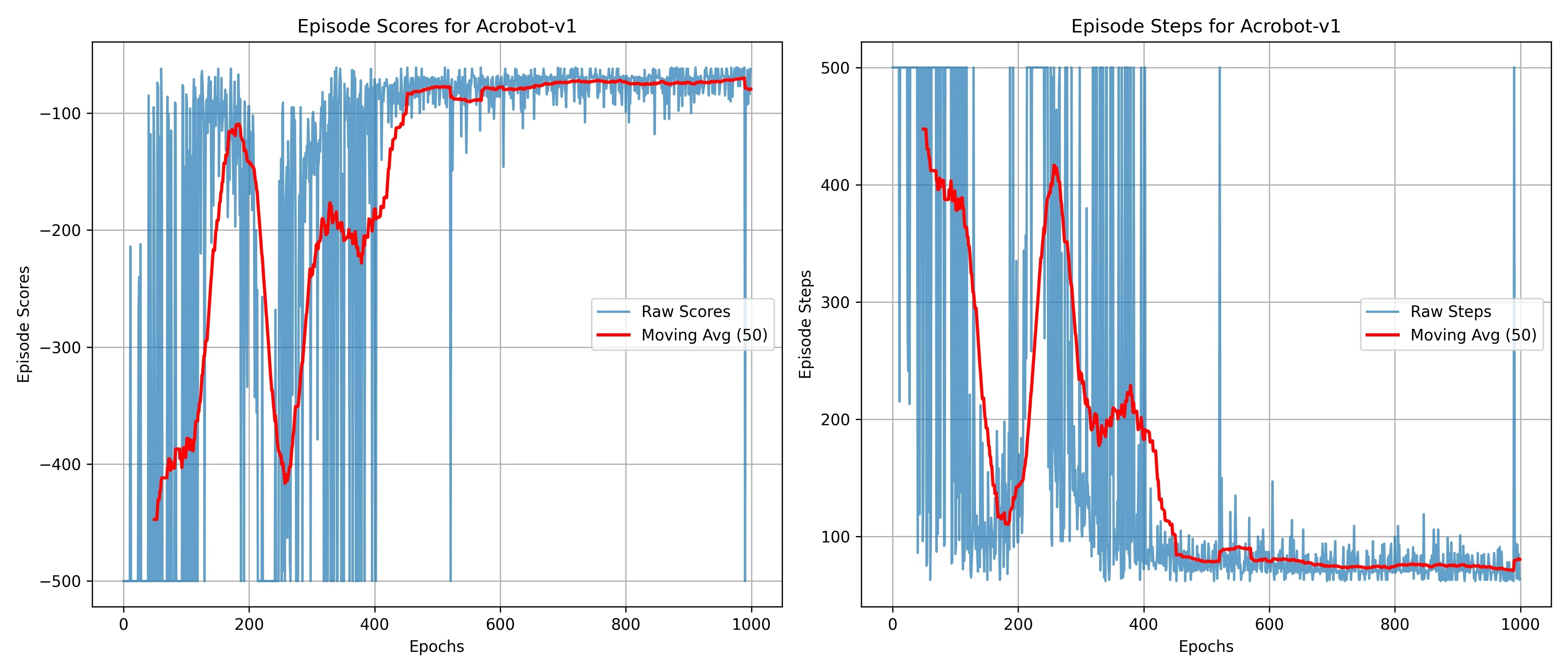
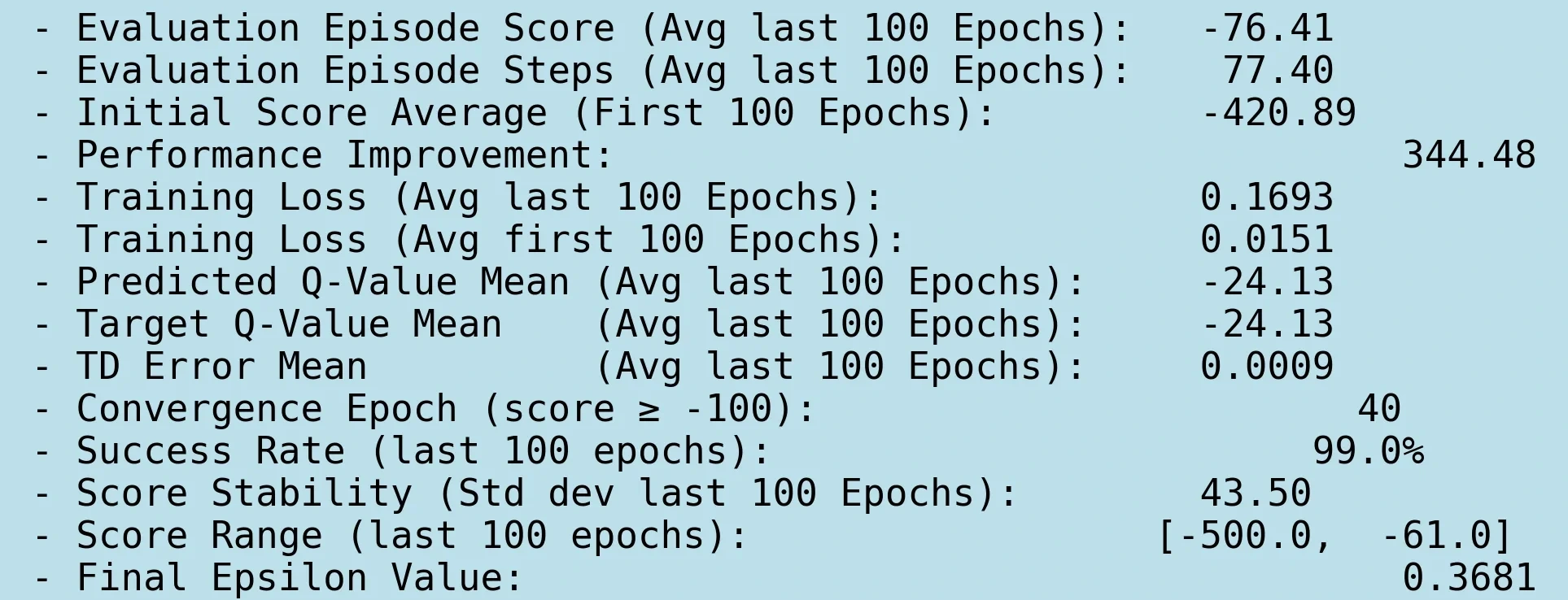
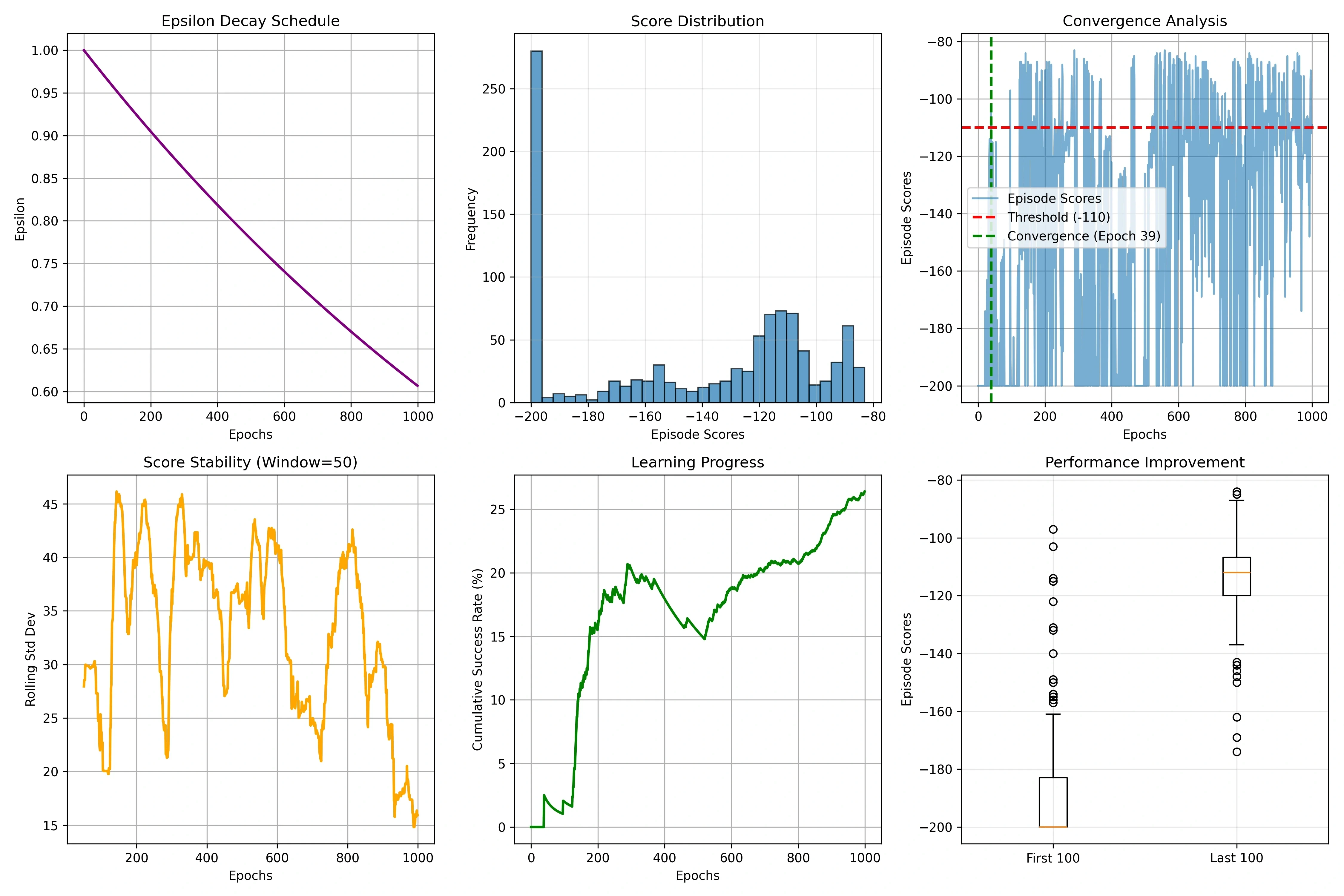
On Acrobot-v1, DQN showed excellent performance in stark contrast to its CartPole results. Figure 5 shows that conservative epsilon decay (1.0→0.3681, rate 0.999) enabled thorough exploration of the complex pendulum dynamics.
Convergence came surprisingly fast, at epoch 40, and the cumulative success rate reached 99%. Despite the 6-dimensional state space and complex swing dynamics, DQN learned the optimal policy quickly.
The score distribution shifted dramatically from early failures around -500 (a -1 reward for all 500 steps) to performance concentrated near the optimal range of -100. This means the agent learned an efficient swing strategy and reaches the goal within about 100 steps.
Figure 6 shows early training instability with a loss spike near epoch 200, but robust convergence follows. The Q-value stabilized at -24.13 with perfect alignment between prediction and target estimates, confirming stable value function learning.
The exceptionally low TD error (0.0009) shows the absence of overestimation bias. This suggests that the overestimation problem observed in CartPole shows up differently depending on the environment. My analysis is that Acrobot's dense negative reward structure led to stable learning.
Figure 7 shows rapid improvement within 150 epochs, with episode length efficiently dropping from 500 to 60-100 steps while keeping high scores. The final metrics in Figure 8 quantify the excellent performance: the average score of -76.41 represents a 344.48-point improvement, validating DQN's effectiveness when the environment's characteristics match the algorithm's strengths.
MountainCar-v0 Results
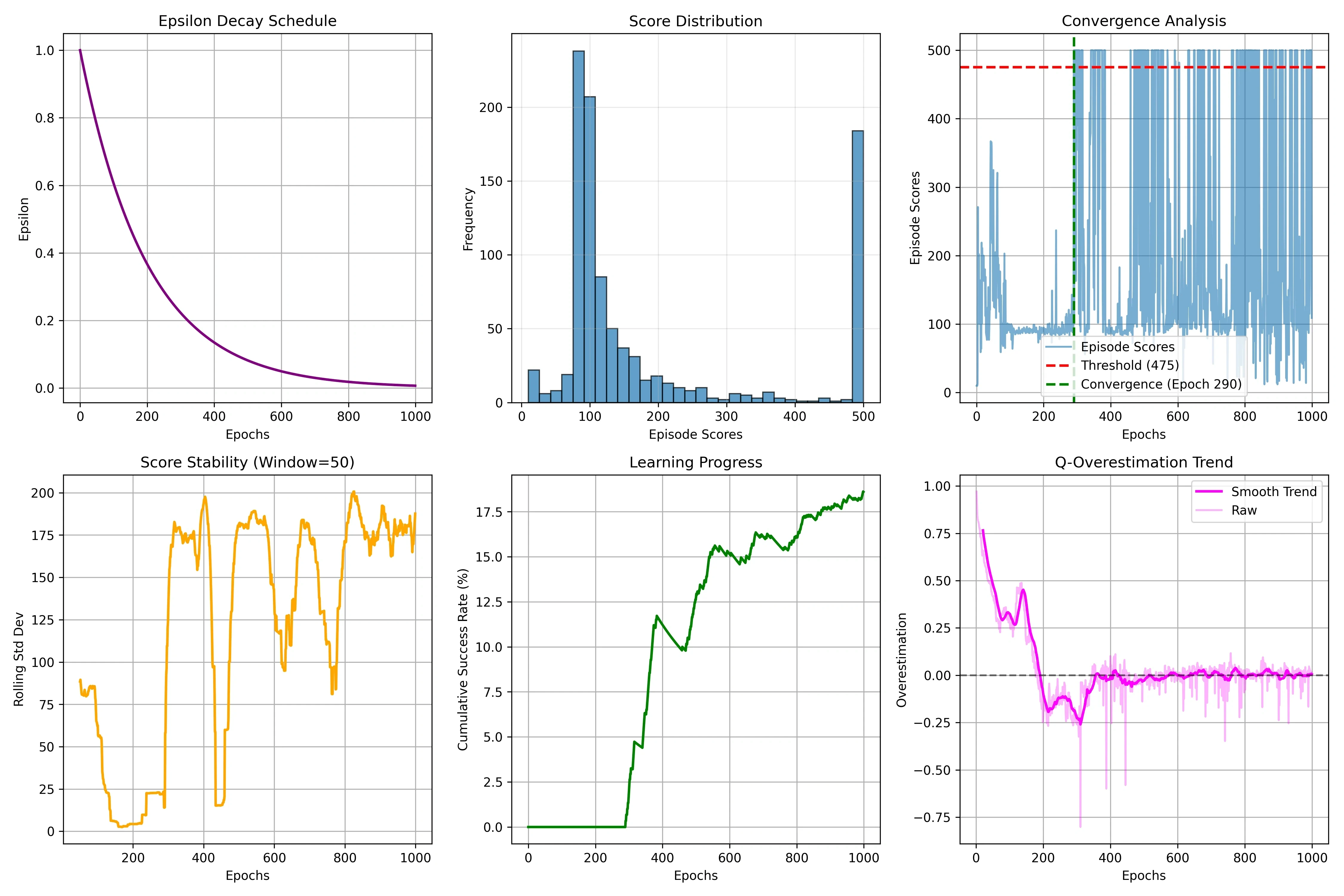
MountainCar-v0 exposes DQN's fundamental limits in sparse-reward environments. Figure 9 shows the most conservative exploration strategy (epsilon: 1.0→0.6068, rate 0.9995) to cope with the sparse-reward challenge, but the cumulative success rate stayed at 30%.
A bimodal score distribution clustered around -200 and -110 is observed. -200 means complete failure to reach the goal across all 200 steps, and around -110 means successfully reaching the goal. This indicates that the right momentum-building strategy is discovered intermittently but not reproduced consistently.
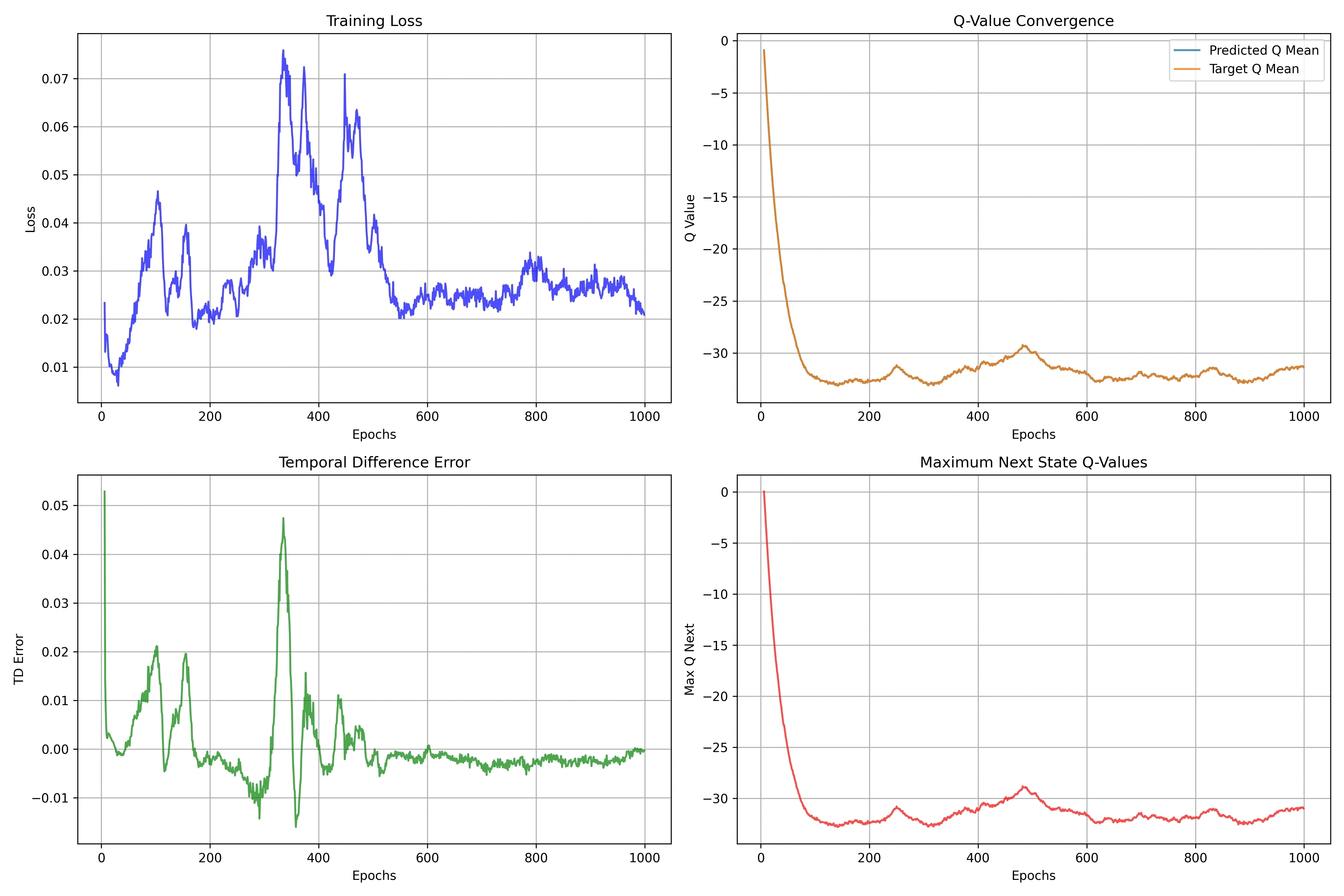
Figure 10 shows paradoxical training stability, where low loss (about 0.02) masks a fundamental learning difficulty. The Q-value stayed consistently low (-31.92) with perfect prediction-target alignment, confirming algorithmic stability without meaningful progress.
This shows a critical limitation of vanilla DQN in sparse-reward settings: numerical convergence without discovering a solution to the task. The network wrongly learns that "circling in place at the bottom of the valley" is the best it can do, and this wrong policy stabilizes with a low TD error and does not improve.
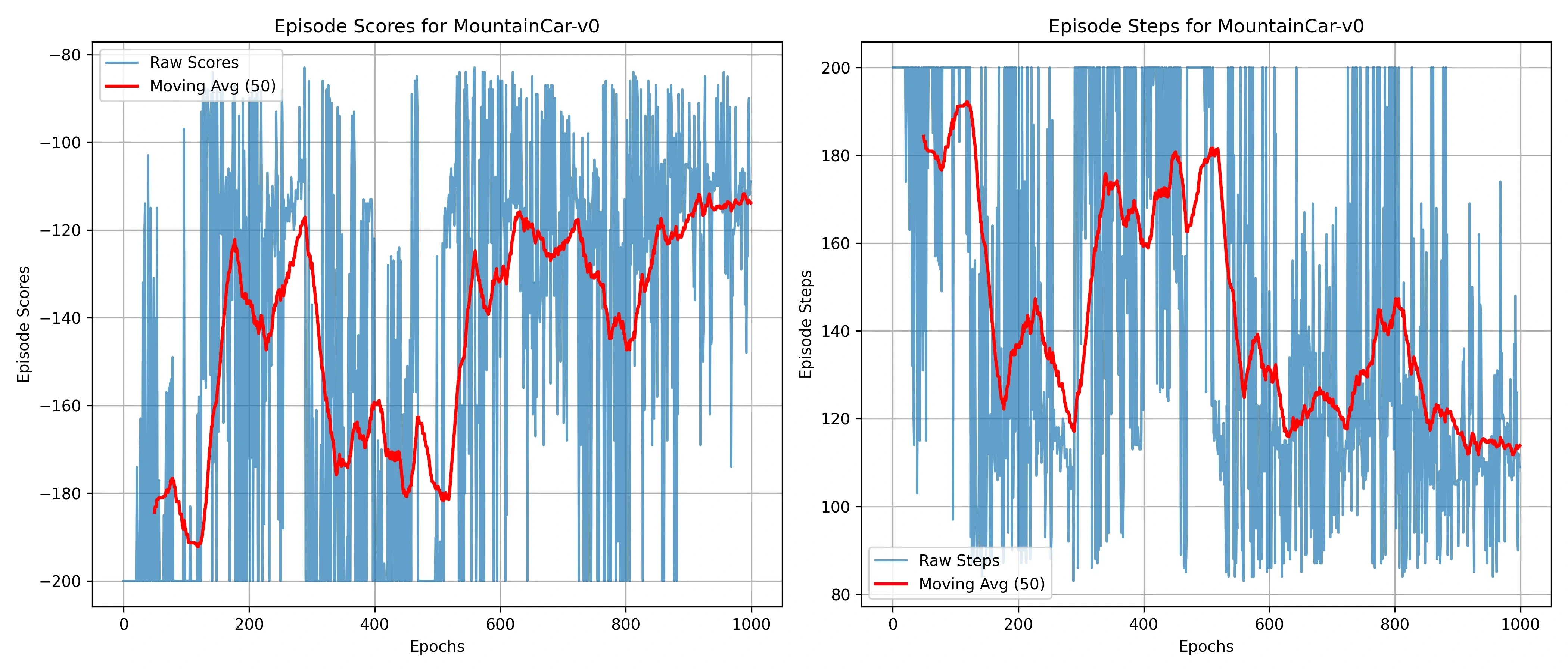
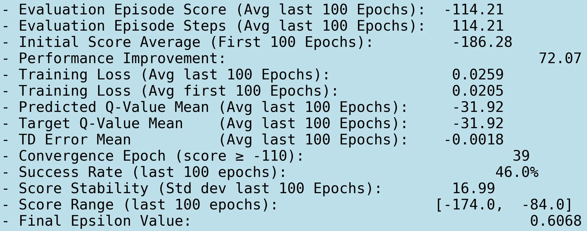
Figure 11 shows gradual improvement in episode length without corresponding goal achievement, revealing an agent that alternates between failing to build momentum and partial success. The final metrics in Figure 12 quantify the limited success: a 46% success rate and a modest 72.07-point improvement show that the algorithm cannot overcome the sparse-reward pathology with hyperparameter tuning alone.
Overall DQN Analysis
The three environments reveal distinct failure modes and capabilities of vanilla DQN.
CartPole's poor performance (12% success rate) stems from overestimation bias. The operator systematically inflates Q-values, causing suboptimal policy updates and a fragile policy. The single-network architecture creates a feedback loop that amplifies estimation errors, resulting in high-variance execution despite numerical convergence.
Acrobot's exceptional performance (99% success rate) shows that environment characteristics, not complexity, determine algorithm performance. The dense negative feedback structure enables stable Q-learning updates, and the deterministic dynamics reduce destabilizing stochastic effects. This environment fits DQN's algorithmic assumptions well.
MountainCar's failure (46% success rate) indicates a sparse-reward pathology, in which TD learning struggles with delayed outcomes and long-term dependencies. The environment requires trajectory-level planning and momentum coordination beyond DQN's Markovian action selection framework. Uniform experience replay dilutes the rare successful experiences among abundant failures, hindering effective policy improvement.
These results provide the motivation for implementing Double DQN, specifically to address the overestimation bias observed in CartPole. However, MountainCar's fundamental sparse-reward challenge suggests that a more sophisticated approach is needed, beyond the architectural improvement of Double DQN.
4. Double DQN Implementation
What Is Double DQN?
Double DQN is an algorithm proposed by van Hasselt et al. in 2016 that addresses DQN's Q-value overestimation problem. I analyzed the cause of this problem and its solution mathematically.
Mathematical Analysis of the Overestimation Problem
DQN's target computation:
The problem lies in the max operator. Suppose the Q-value estimates have uniformly distributed noise ε around the true values:
The expected value of the max operation:
By Jensen's inequality, the expected value of the max is greater than or equal to the max of the expected values. Therefore, even if the noise has zero mean, the max operation causes overestimation.
Double DQN's Solution
The key idea is to separate action selection from action evaluation:
DQN target:
→ The same network (θ⁻) handles both action selection and evaluation
Double DQN target:
→ The online network (θ) selects the action, and the target network (θ⁻) evaluates it
With this separation, the same noise does not affect selection and evaluation at the same time, which reduces overestimation.
Double DQN Implementation Details
Modifying the Training Method
I modified the train method so that the online network selects the action and the target network evaluates that action's Q-value.
Analysis of the Key Change
The difference from DQN is just two lines:
is the key. It extracts the action index selected by the online network from the target network's Q-values.
Double DQN Results
CartPole-v1 Results
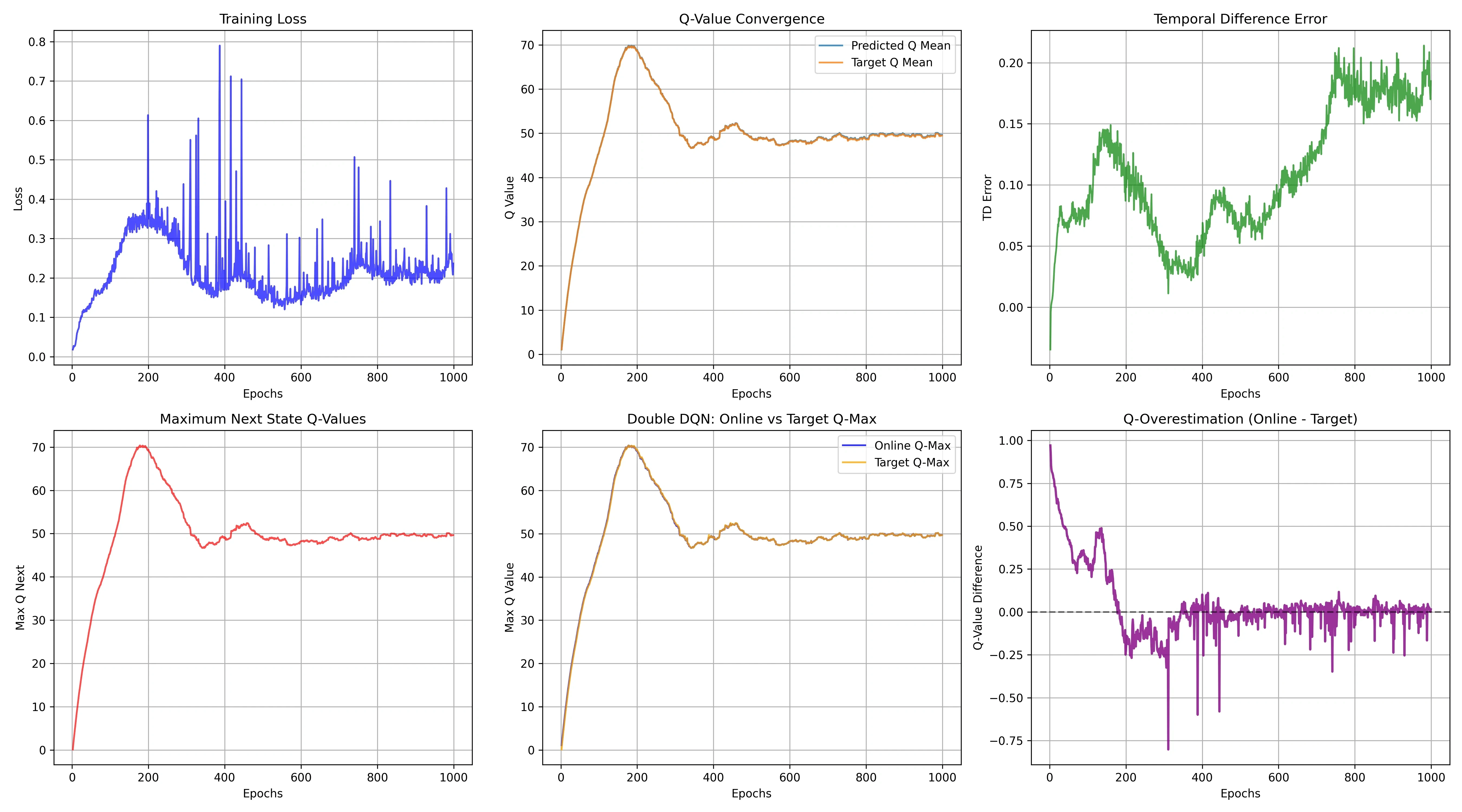
On CartPole-v1, Double DQN shows measurable improvement over vanilla DQN, mainly through effective reduction of overestimation bias. Figure 13 shows the core overestimation trend dropping from 0.447 to nearly 0, validating the algorithm's key theoretical advantage.
Confirming numerically that the overestimation reduction mechanism actually works is a meaningful result. Where Q_pred - Q_target tended to accumulate positive values in DQN, it stabilizes near 0 in Double DQN.
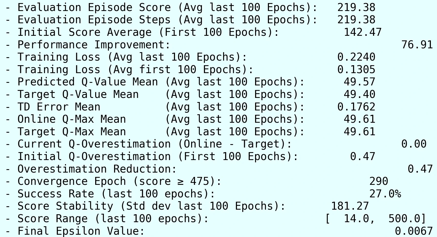
However, this improvement came with delayed convergence (epoch 290 vs. 100 for vanilla DQN). There is a trade-off in which more conservative value estimates slow learning in the early exploration phase. Without optimistic Q-values, the agent has less incentive to try new actions.
The final average score improved to 219.38 (43.9% of optimal), a 23% performance gain over vanilla DQN, but the success rate of 27% is still suboptimal.
Figure 14 shows more stable training dynamics, with the predicted and target Q-values converging tightly around 49.5, demonstrating reduced overestimation artifacts. The training loss stabilized around 0.22 with less variability than vanilla DQN.
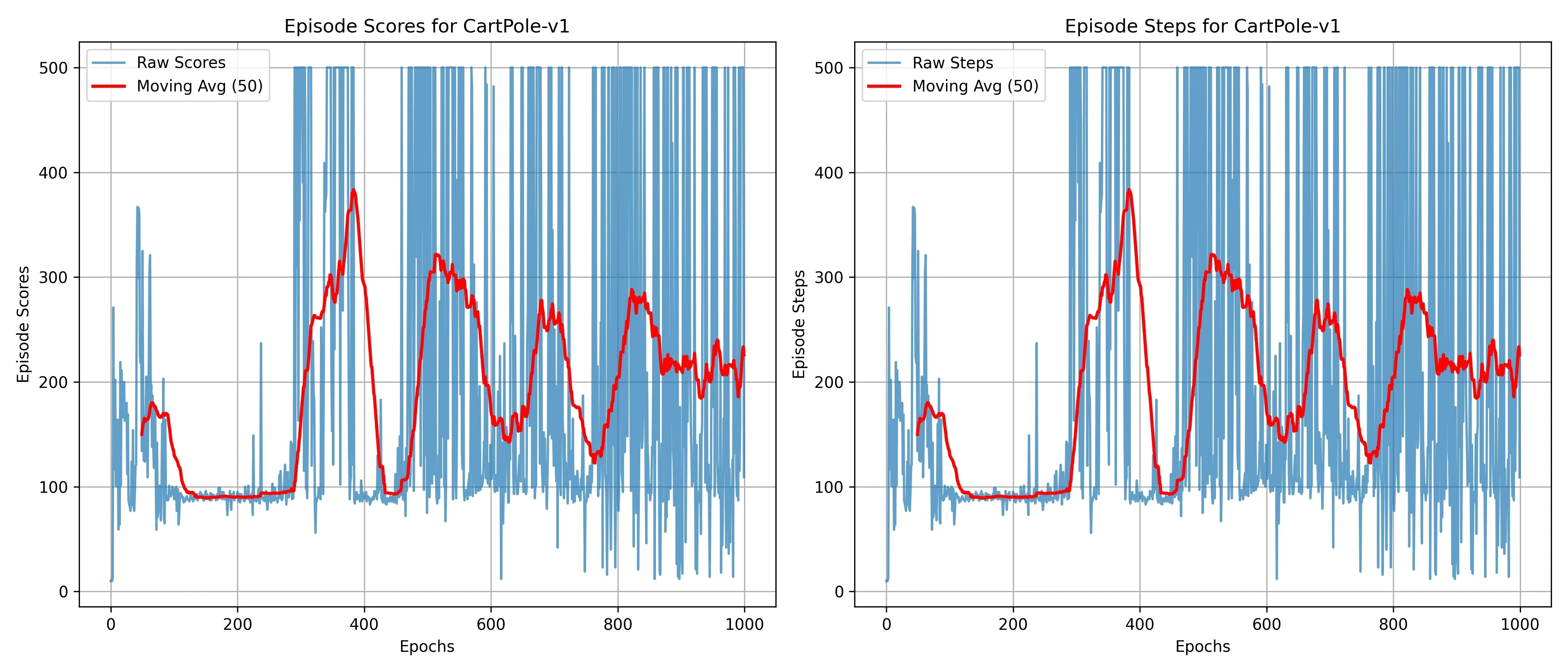
Figure 15 shows an improved learning pattern with fewer sudden performance collapses, but oscillating behavior persists throughout training. Despite the elimination of overestimation bias shown in Figure 16, the high score variance (σ=181.27) indicates that the underlying policy stability problem was not solved.
This is an important finding. It confirms that overestimation bias is only one component of vanilla DQN's limitations on CartPole, and that other factors (e.g., high variance in policy gradients, limited network capacity) also affect performance.
Acrobot-v1 Results
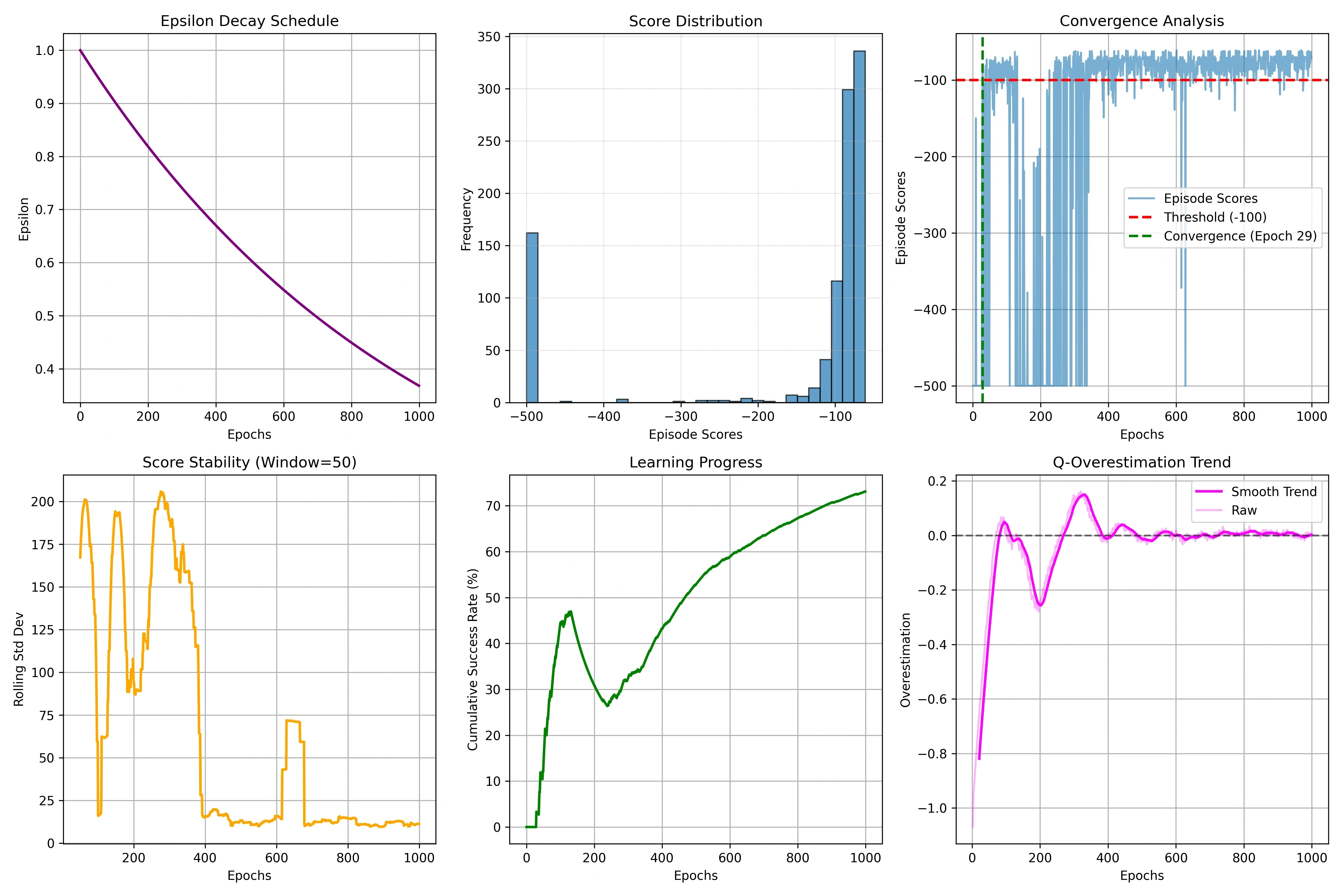
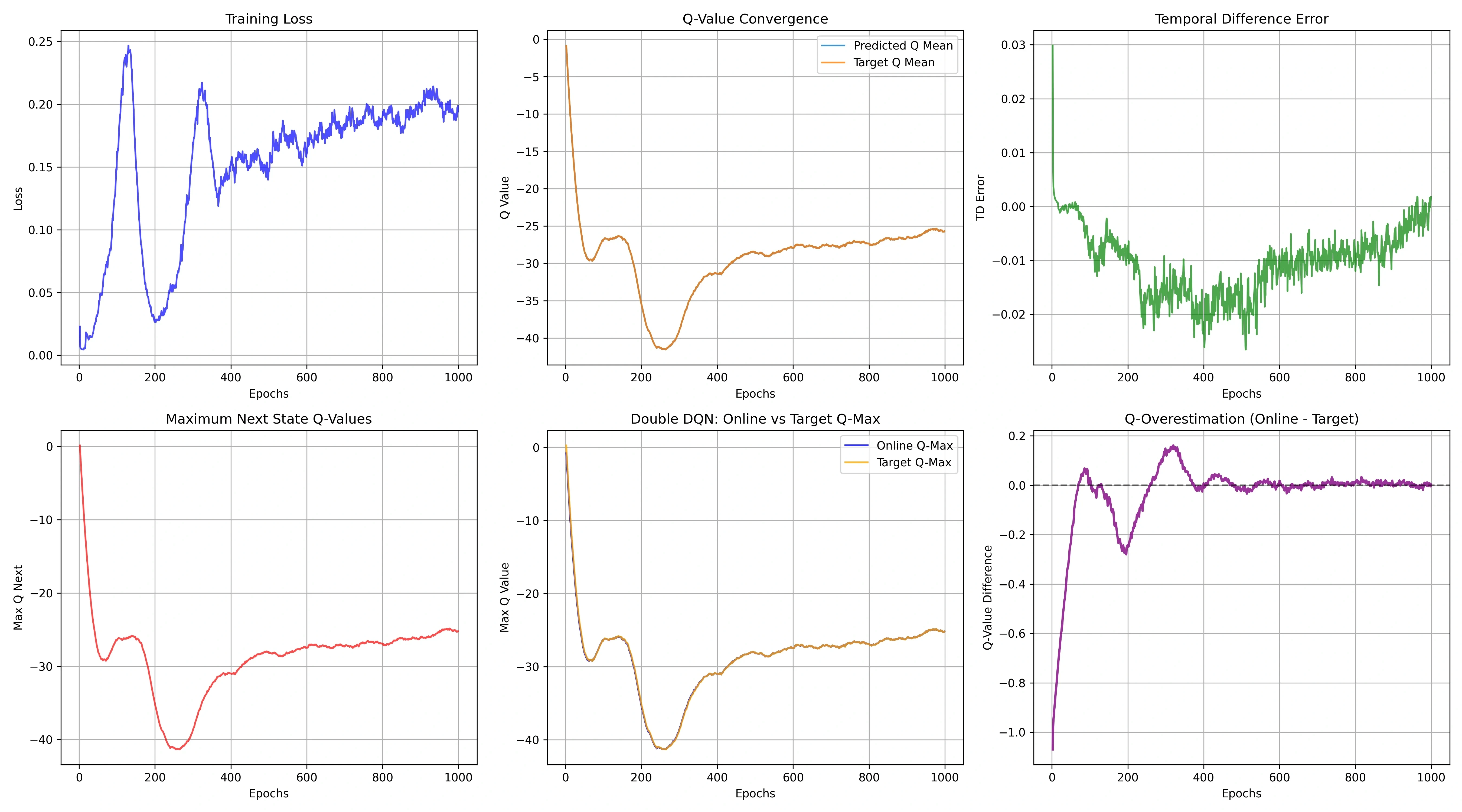
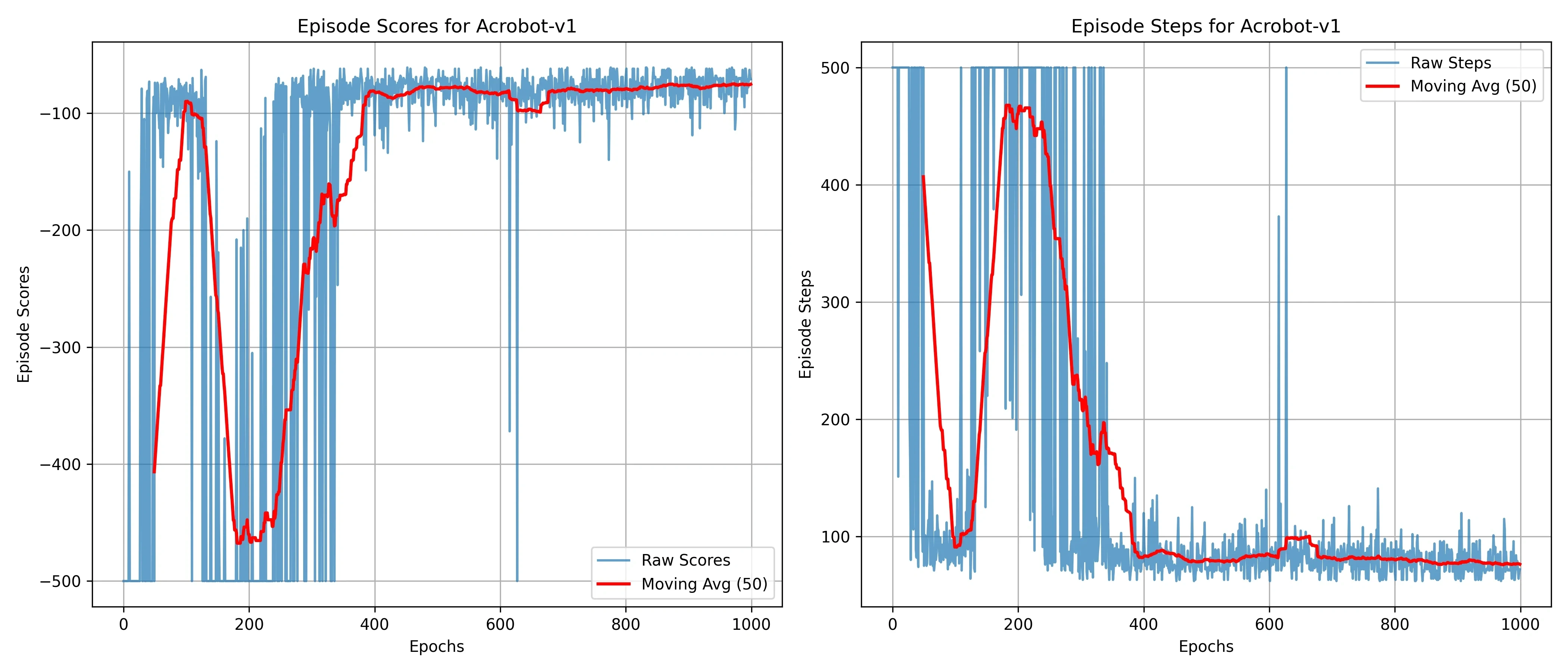
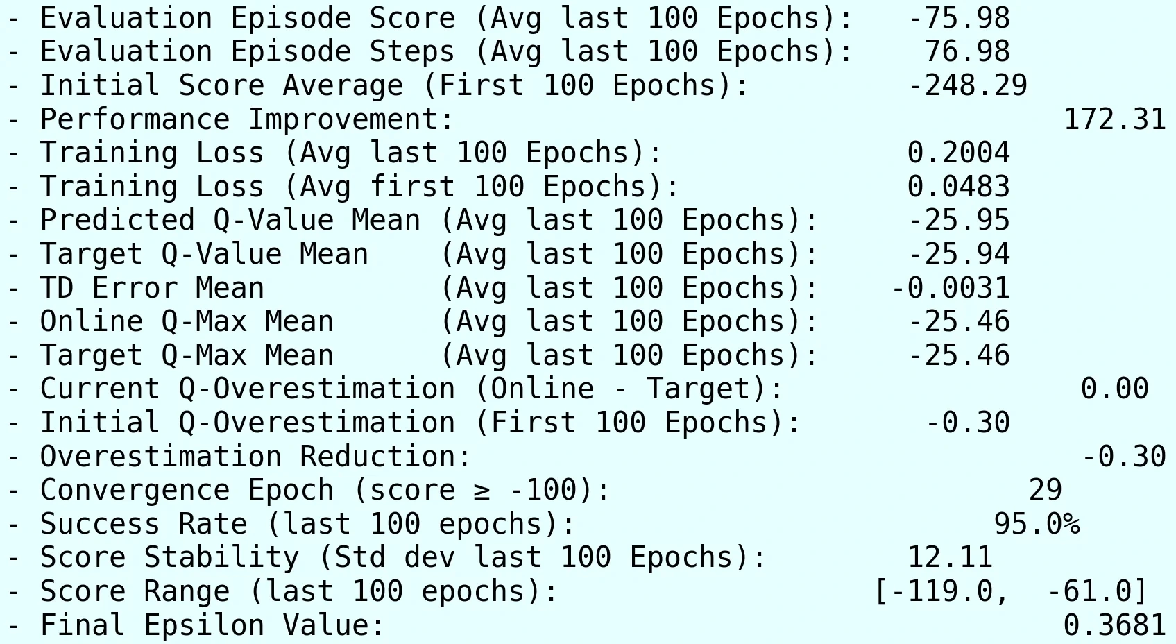
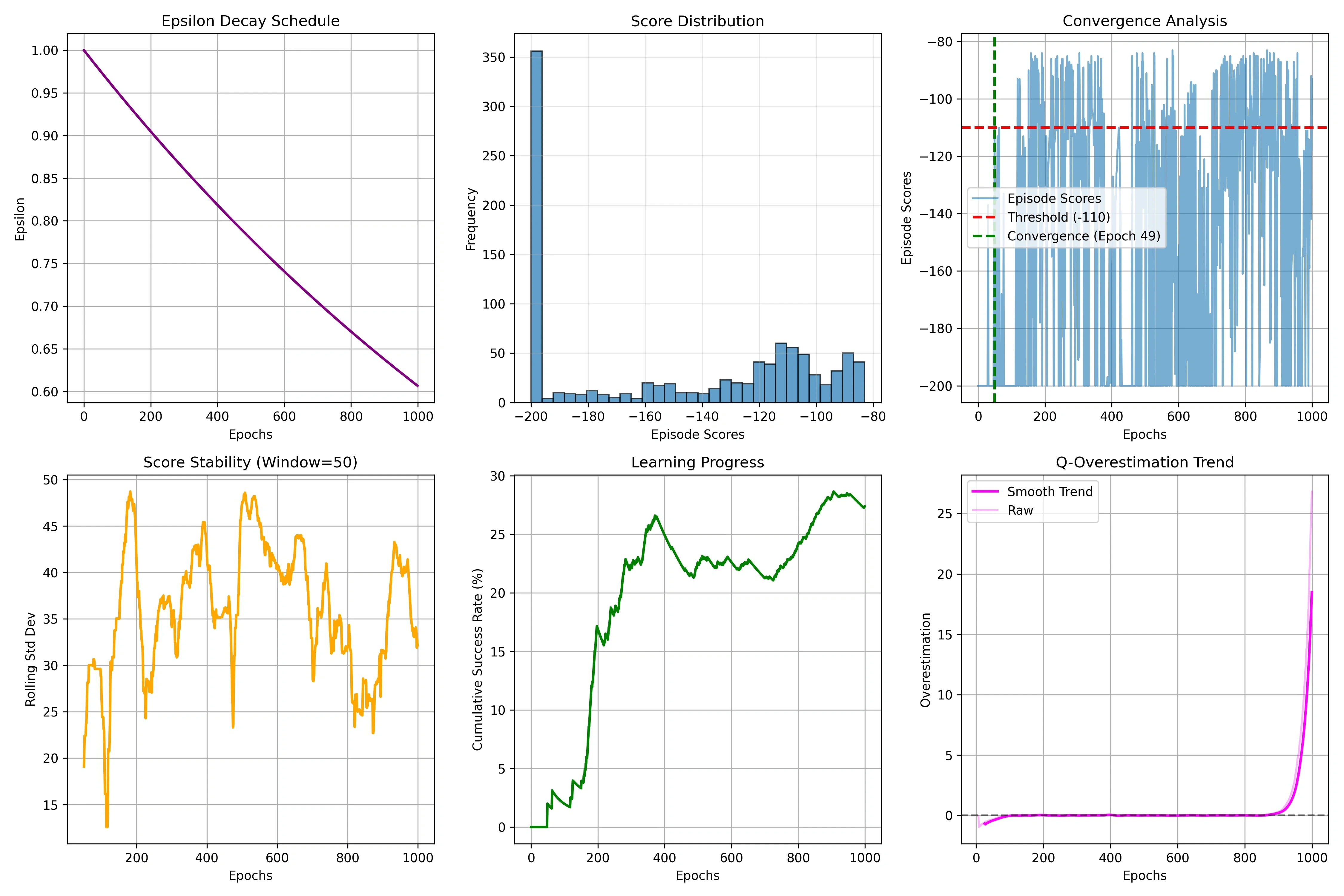
On Acrobot-v1, Double DQN maintained excellent performance while providing improved stability compared to vanilla DQN. Figure 17 shows fast convergence with a 95% success rate at epoch 29, confirming that the algorithm keeps its effectiveness in environments with a suitable reward structure.
The overestimation trend shows an initial bias of about 0.2 stabilizing near 0, confirming Double DQN's theoretical advantage even in an environment where vanilla DQN already performed well. It is an interesting finding that overestimation existed even though DQN reached a 99% success rate. In this environment, overestimation did not greatly affect performance, but Double DQN was confirmed to reduce it.
Figure 18 shows stable training dynamics, with the Q-value converging to -25.95 and an exceptionally low TD error (-0.0031). The overestimation control mechanism worked effectively without hurting the fast learning characteristics that made vanilla DQN successful in this environment.
Figure 19 shows the characteristic pattern of rapid improvement within 150 epochs, with efficient episode completion maintained throughout training. The final metrics in Figure 20 show performance nearly identical to vanilla DQN (-75.98 vs. -76.41) but with improved stability (score standard deviation: 12.11 vs. 43.5), confirming that Double DQN preserves the algorithm's strengths while adding robustness.
MountainCar-v0 Results
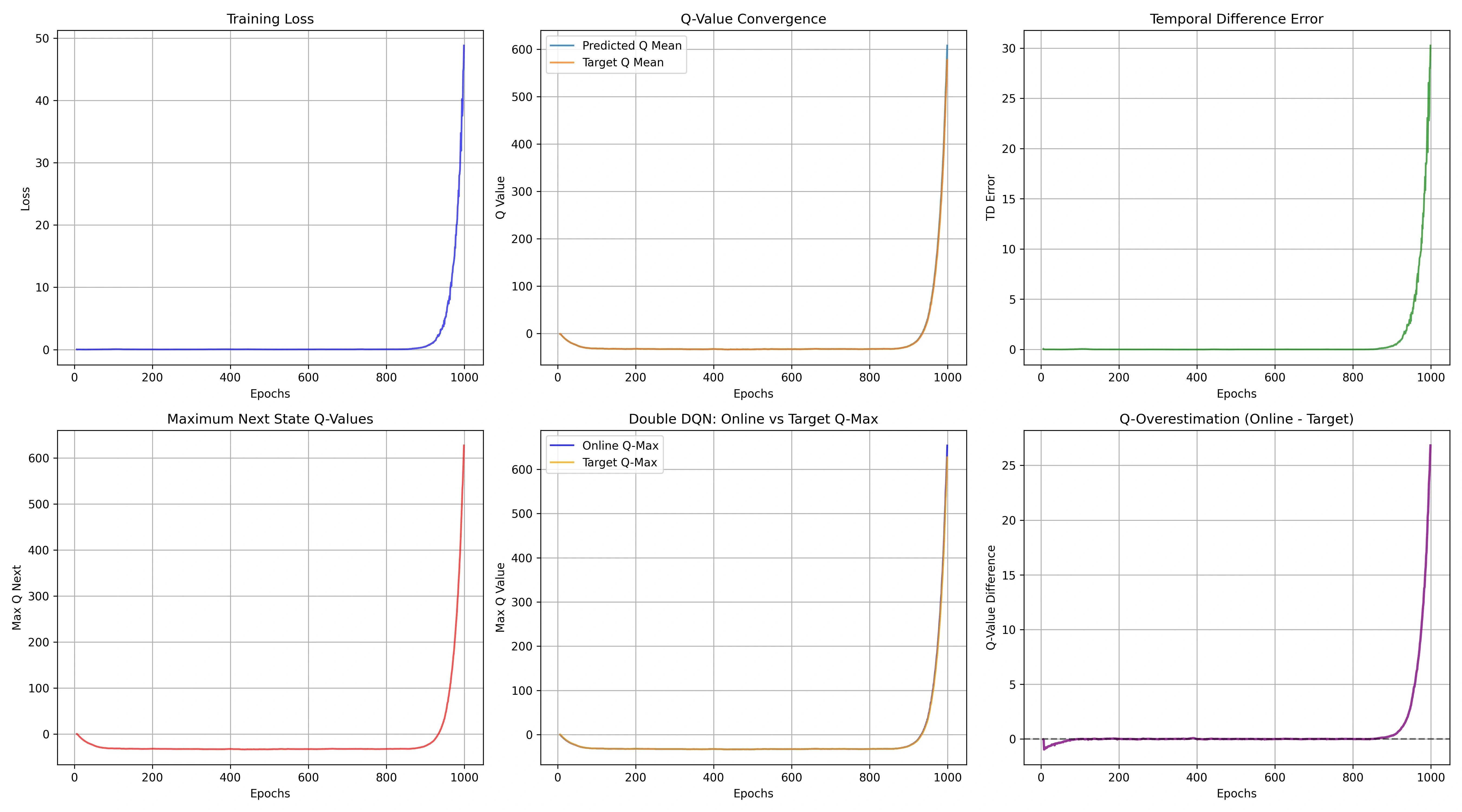
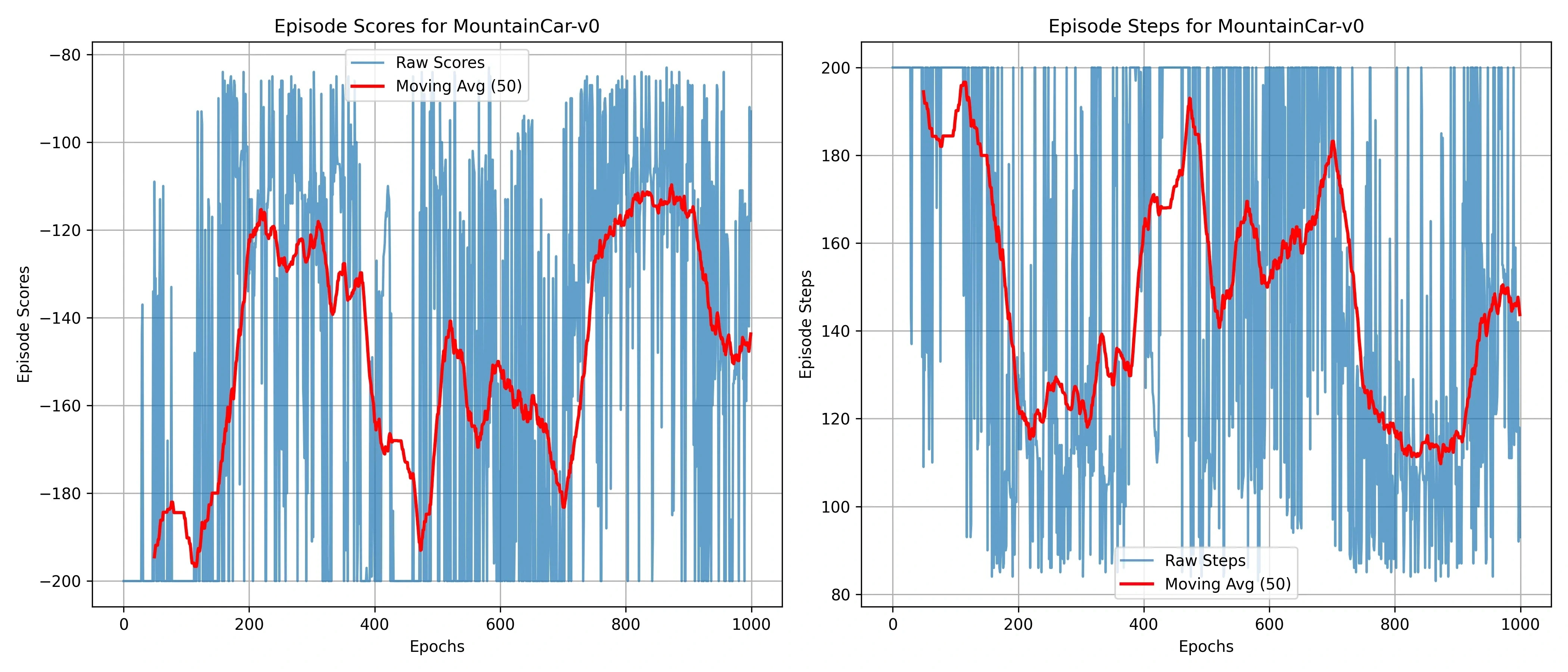
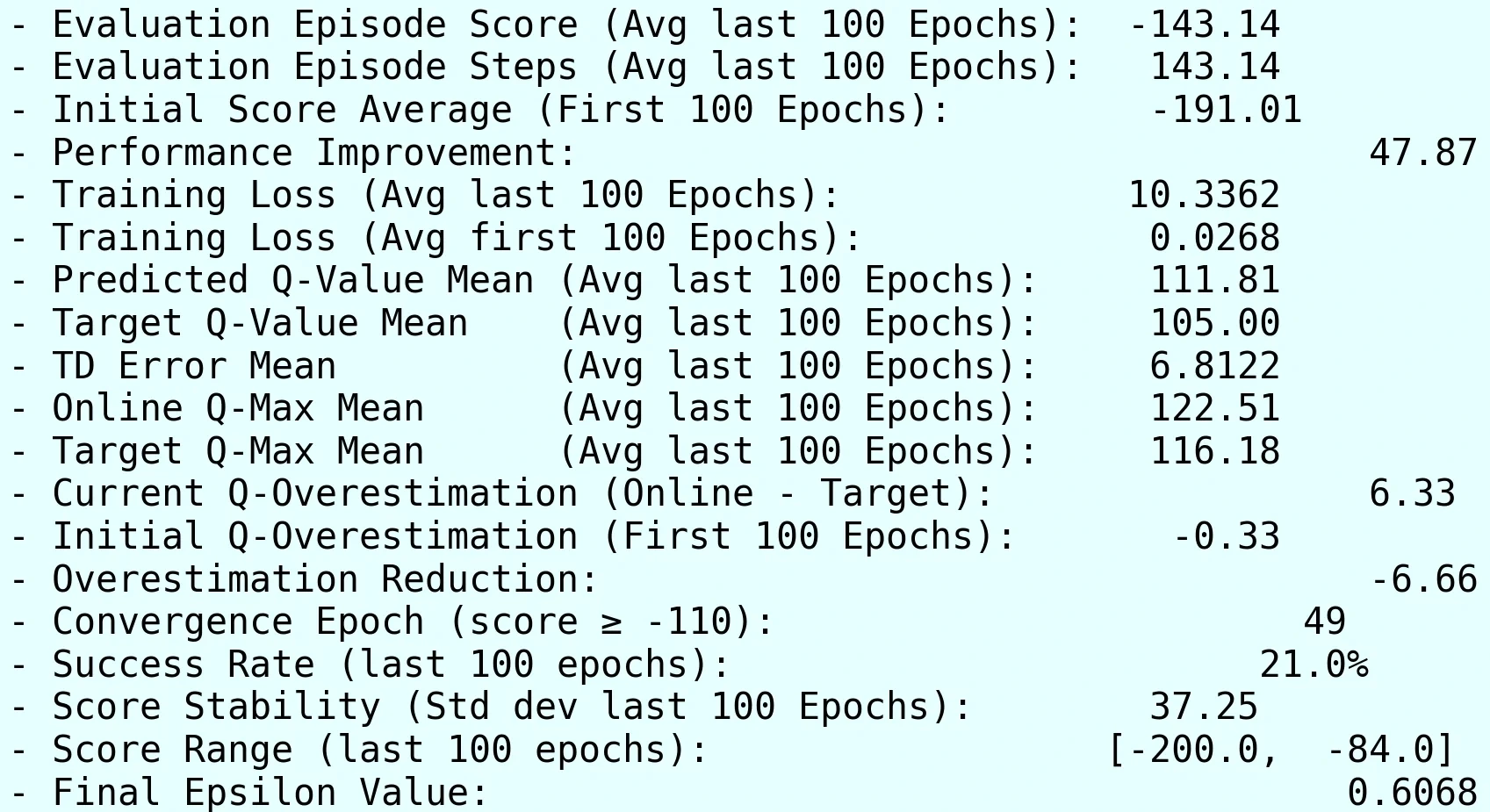
On MountainCar-v0, Double DQN shows marginal improvement in places but failed to overcome the fundamental sparse-reward pathology. More surprisingly, it actually performed worse than DQN.
Figure 21 shows a reduced success rate (21% vs. 46% for vanilla DQN) with late convergence at epoch 49. This exposes a key limitation of Double DQN: more conservative value estimates hinder exploration in sparse-reward environments.
In a sparse-reward environment, the agent receives a meaningful learning signal only when it reaches the goal by chance. DQN's optimistic Q-value estimates provide an incentive that says "worth a try," which encourages exploration. Double DQN's conservative estimates, by contrast, send a signal that says "not worth trying," which suppresses exploration.
The final score of -143.14 represents worse performance than vanilla DQN (-114.21), confirming the algorithm's limitation when overestimation bias is not the main bottleneck.
Figure 22 shows problematic training dynamics, with considerably higher loss values and unstable Q-value estimates reaching extreme values (>600), indicating algorithmic difficulty in the sparse-reward setting. The overestimation reduction mechanism appears counterproductive in an environment that needs optimistic exploration to discover rare successful trajectories.
Figure 23 shows a performance pattern worse than vanilla DQN, with more erratic score oscillation throughout training. The metrics in Figure 24 confirm inferior performance across several dimensions, demonstrating that Double DQN's conservative approach can hinder learning when the environment requires aggressive exploration to overcome the sparse-reward challenge.
Overall Double DQN Analysis
Double DQN's results across the three environments reveal environment-dependent algorithm effectiveness and offer important insights into deep reinforcement learning design principles.
CartPole-v1 shows a clear but limited benefit from reduced overestimation bias, validating the theoretical framework with a 23% performance gain while revealing additional stability challenges that need complementary solutions. The high variance that persists despite the bias correction suggests that policy fragility stems from several algorithmic limitations, not overestimation alone.
Acrobot-v1 demonstrates Double DQN's ability to strengthen already-successful performance with improved stability, without sacrificing learning efficiency. The algorithm keeps a 95% success rate while cutting score variance by 3x, showing that reducing overestimation bias provides meaningful benefits even in environments where vanilla DQN performs acceptably.
MountainCar-v0 exposes a critical limitation: in sparse-reward environments where optimistic value estimates drive needed exploration, reducing overestimation bias can be counterproductive. The worse performance (21% vs. 46% success rate) confirms that algorithm modifications must match the environment's requirements, and that conservative value estimates can hinder the discovery of rare successful trajectories.
This result is an important finding that runs against the common belief that "Double DQN is always better than DQN."
5. PER (Prioritized Experience Replay) Implementation
What Is PER?
PER (Prioritized Experience Replay) is a technique proposed by Schaul et al. in 2016 that gives higher priority to experiences with large TD errors, so the agent learns more often from important transitions.
The Problem with Uniform Sampling
Basic DQN's Experience Replay samples uniformly from the buffer:
Problems:
- Rare successful experiences get diluted among abundant failures
- Experiences that are already well learned and experiences that still need learning are treated equally
- Lower learning efficiency
Priority-Based Sampling
A large TD error δ means "the prediction was badly wrong" = "this still needs to be learned." PER takes advantage of this:
- α=0: uniform sampling (basic Experience Replay)
- α=1: fully prioritized sampling
Importance Sampling Correction
Prioritized sampling distorts the distribution, which introduces bias. Importance Sampling weights are used to correct it:
- β=0: no correction
- β=1: full correction
β starts low early in training and is gradually increased to 1. Fast learning matters early on, while accurate convergence matters later.
PER Implementation Details
1) Prioritized Replay Buffer Implementation
Implementation Decisions
Why assign maximum priority to new experiences? A new experience has not been used for training yet, so its TD error is unknown. Assigning the maximum priority conservatively guarantees that it is sampled at least once.
Why set a priority cap (1000.0)? If an extremely large TD error occurs, that experience alone may be sampled over and over, biasing training. The cap preserves diversity.
β scheduling strategy Start at β=0.4 and gradually increase to 1.0. Early in training, the bias of prioritized sampling is tolerated for faster learning; later, it is fully corrected for accurate convergence.
2) Per-Environment Hyperparameter Tuning
I tuned the PER parameters to fit the characteristics of each environment.
Rationale for each environment
- MountainCar (α=0.7): in a sparse-reward environment, rare successful experiences matter a lot, so strong priority differentiation is needed
- CartPole (α=0.6): a moderate level of differentiation to keep a balance
- Acrobot (α=0.5): in a dense-reward environment, all experiences are relatively important, so differentiation is low
3) Modifying the Training Method
I modified it to apply the IS weights to the loss and to update priorities after training.
How the IS weights are applied
The per-sample losses are kept with and then multiplied by the weights:
Frequently sampled experiences (high P(i)) get lower weights, reducing their gradient contribution. This corrects the bias of prioritized sampling.
PER Results
CartPole-v1 Results
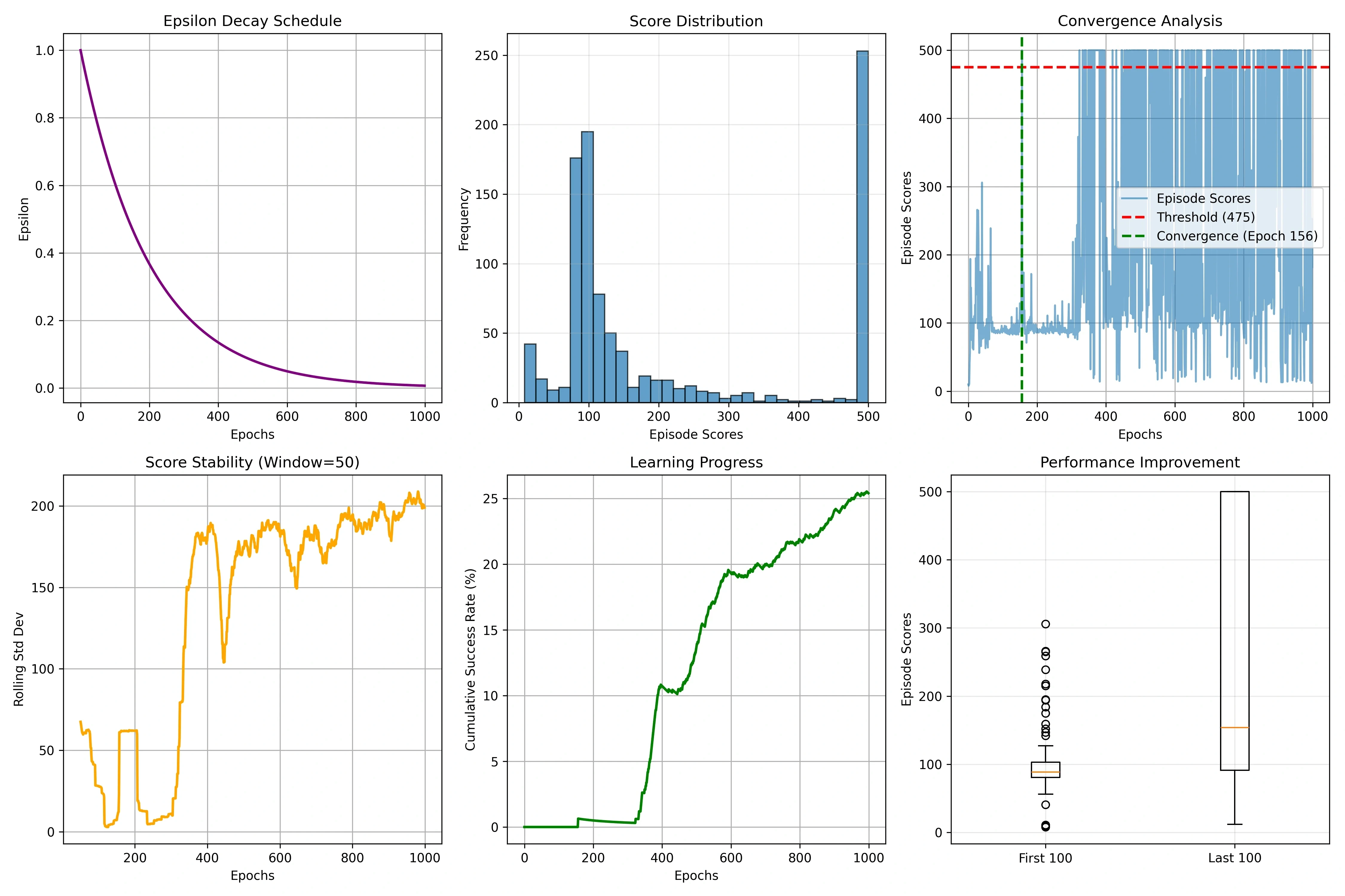
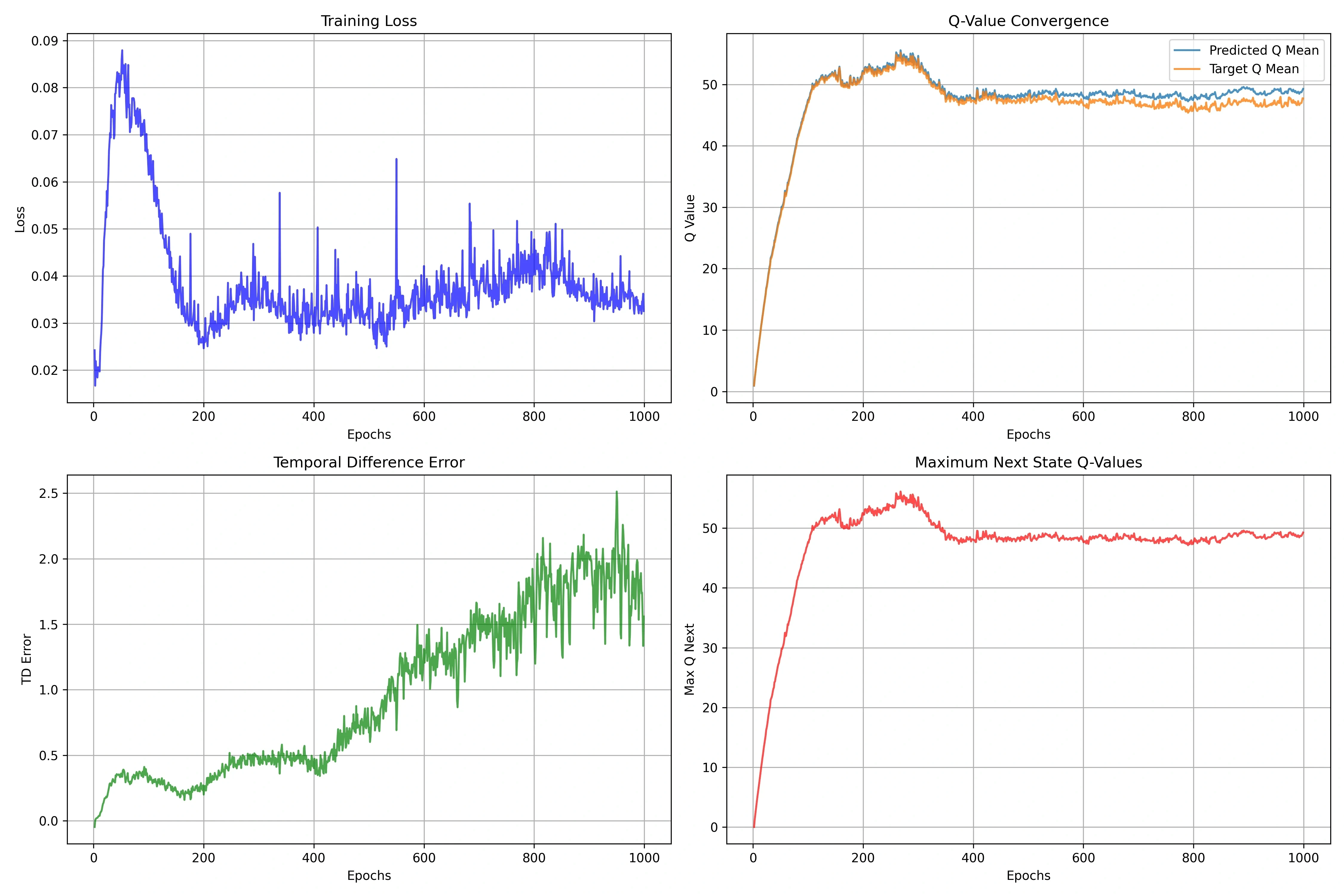
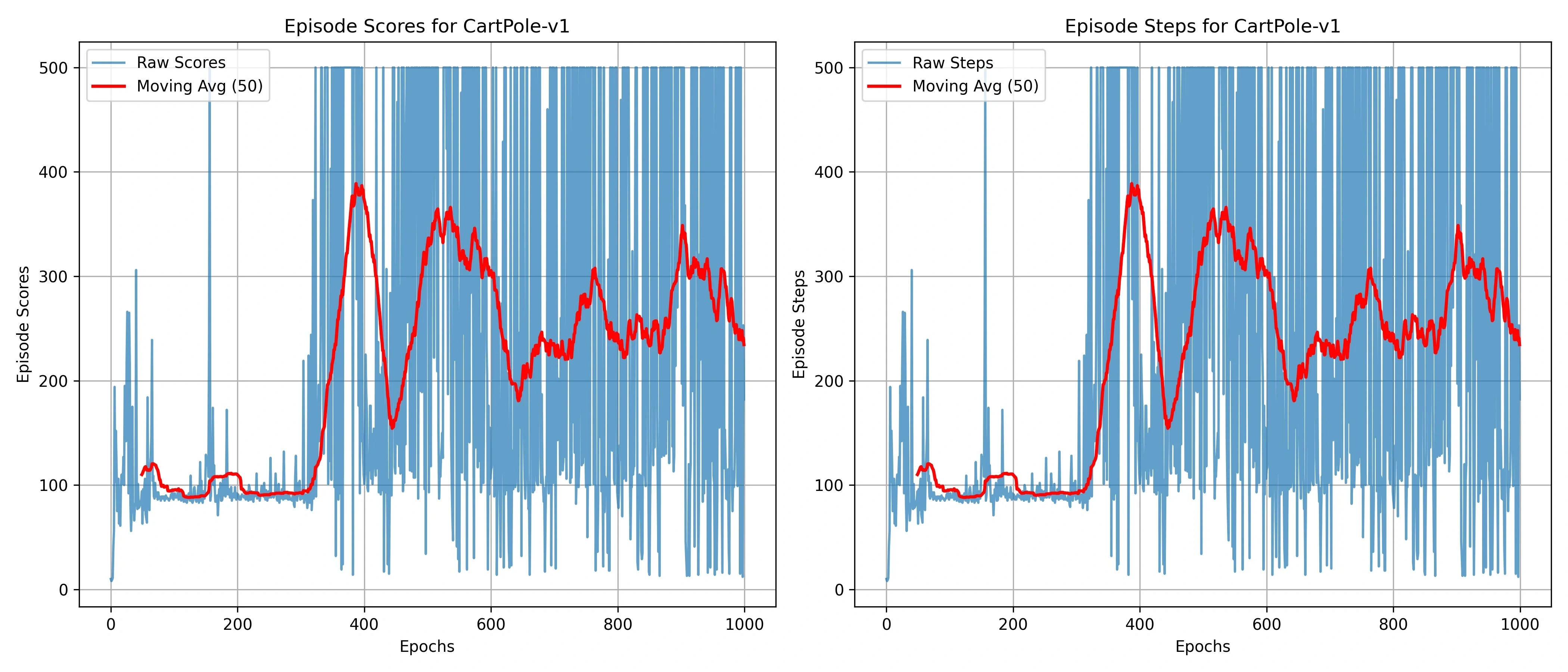
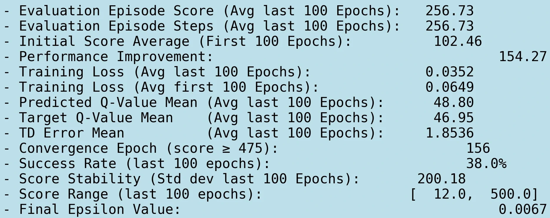
On CartPole-v1, PER achieved the best performance of all tested algorithms, with a final average score of 256.73 (51.3% of optimal) and a 38% success rate.
Figure 25 shows delayed but more stable convergence at epoch 156, with improved learning progress reaching a 25% cumulative success rate. The prioritized sampling mechanism effectively focused learning on transitions with high TD errors (critical moments of recovering from failure or leading to success).
The problem with uniform sampling in CartPole is that 500-step successful episodes and 50-step failed episodes are treated equally. Successful episodes contribute 10x more experiences, but the experiences right before failure (high TD error) matter more for learning. PER effectively reuses these "right before failure" experiences.
Figure 26 shows stable training dynamics, with the Q-value converging around 48.80. The TD error evolution shows a more consistent pattern than vanilla DQN, indicating improved value function approximation.
Figure 27 shows a characteristic learning progression with fewer catastrophic performance drops and more sustained high-performance episodes. Despite the remaining score variance (σ=200.18), the substantial performance gain validates PER's effectiveness at addressing experience replay inefficiency.
Algorithm comparison:
- DQN: 178.13 points (35.6%)
- Double DQN: 219.38 points (43.9%)
- PER: 256.73 points (51.3%)
Acrobot-v1 Results
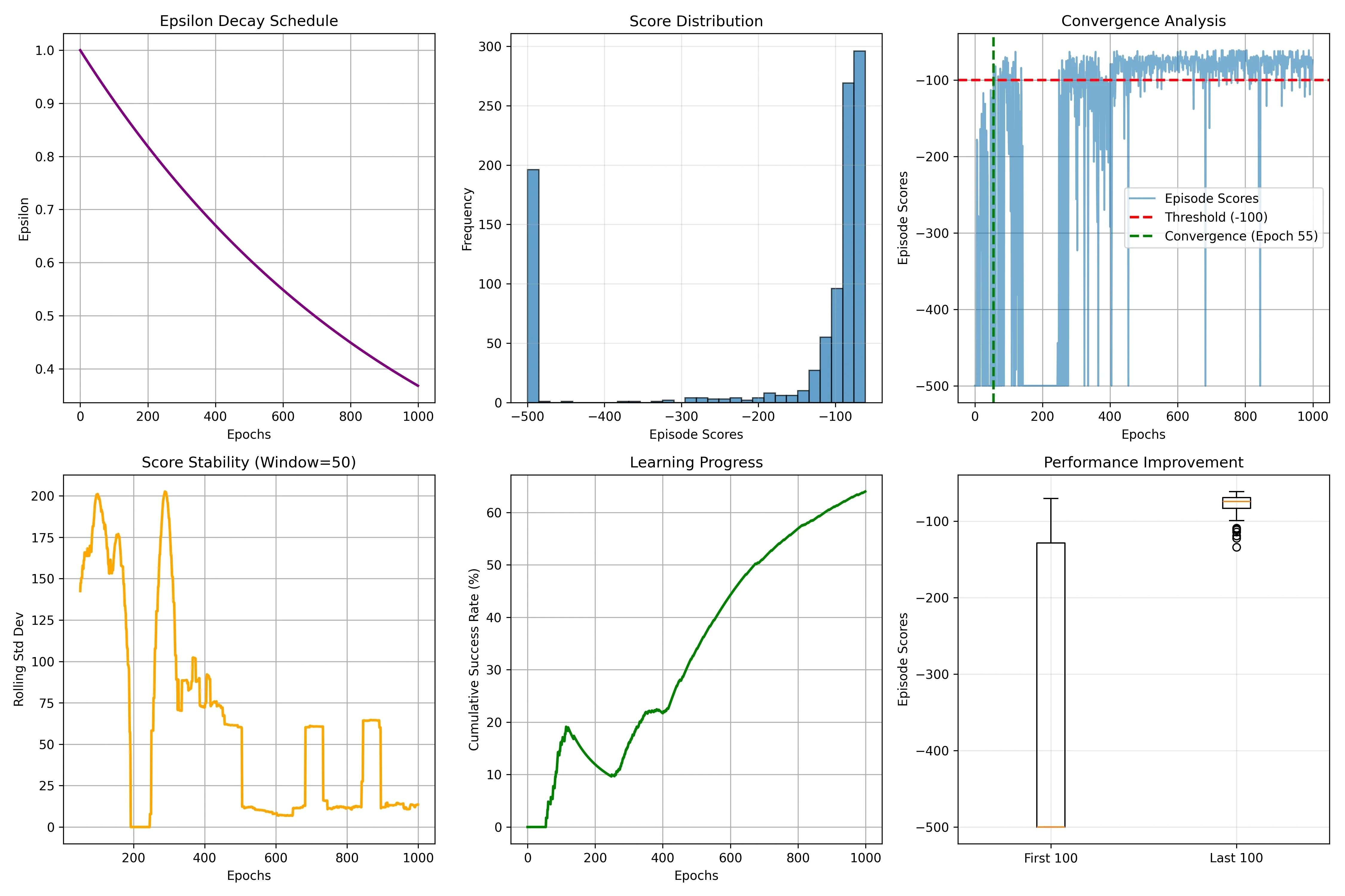
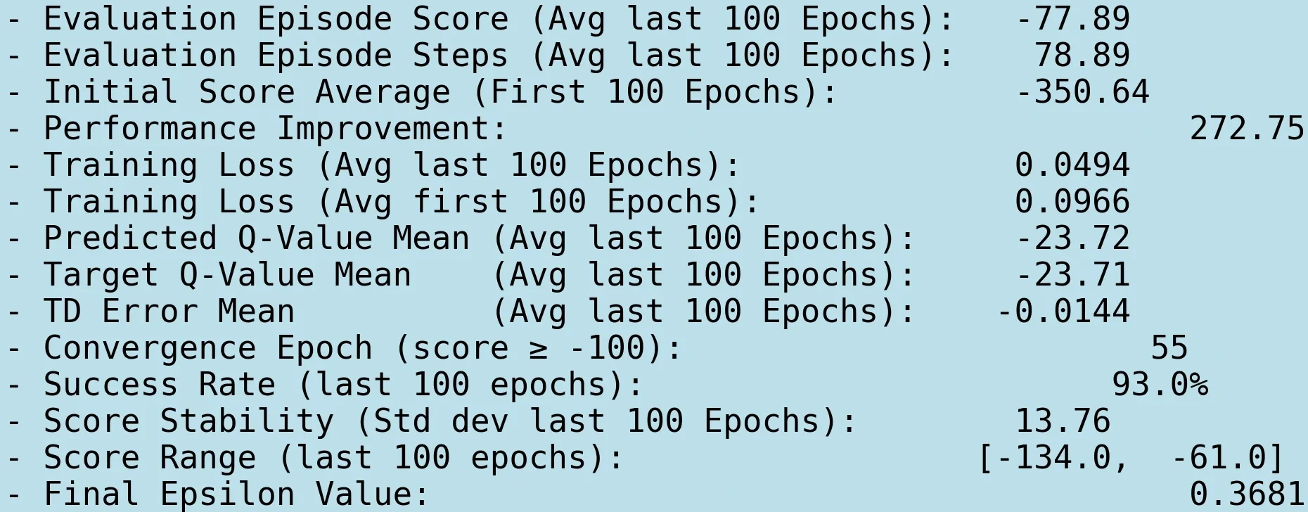
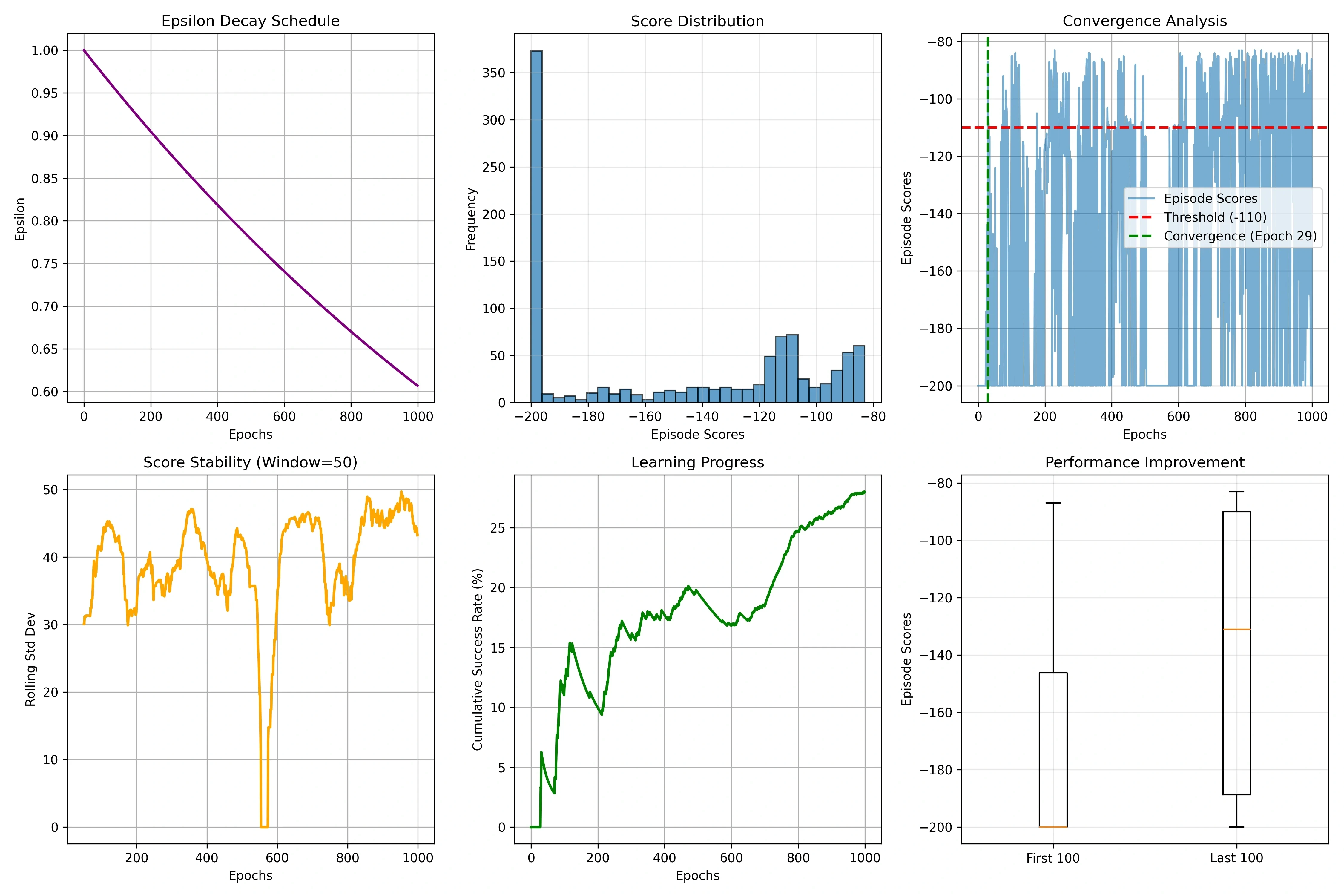
On Acrobot-v1, PER maintained excellent performance while providing improved stability compared to the earlier algorithms. Figure 29 shows fast convergence with a 93% success rate at epoch 55, confirming that prioritized sampling preserves the algorithm's effectiveness in environments with a suitable reward structure.
The final score of -77.89 represents optimal-level performance with improved consistency throughout training. PER's advantage on Acrobot is that it focuses on the critical moments of learning "swing timing." Experiences at the moment the pendulum reaches its highest point have large TD errors, and learning them repeatedly yields an efficient swing policy.
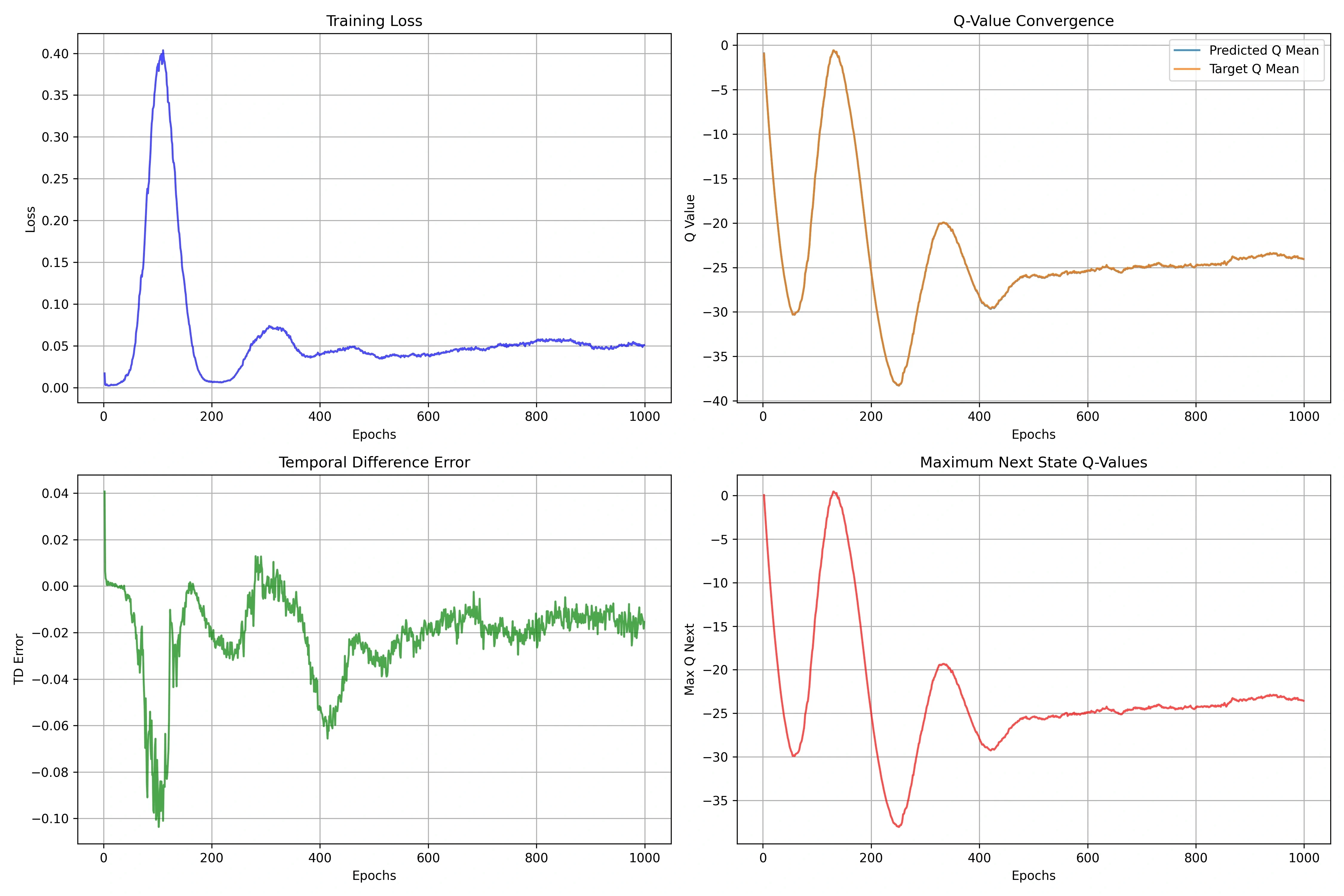
Figure 30 shows stable training dynamics with minimal oscillation and consistent value function convergence around -23.72. The prioritized replay mechanism kept the fast learning characteristics while reducing training variance.
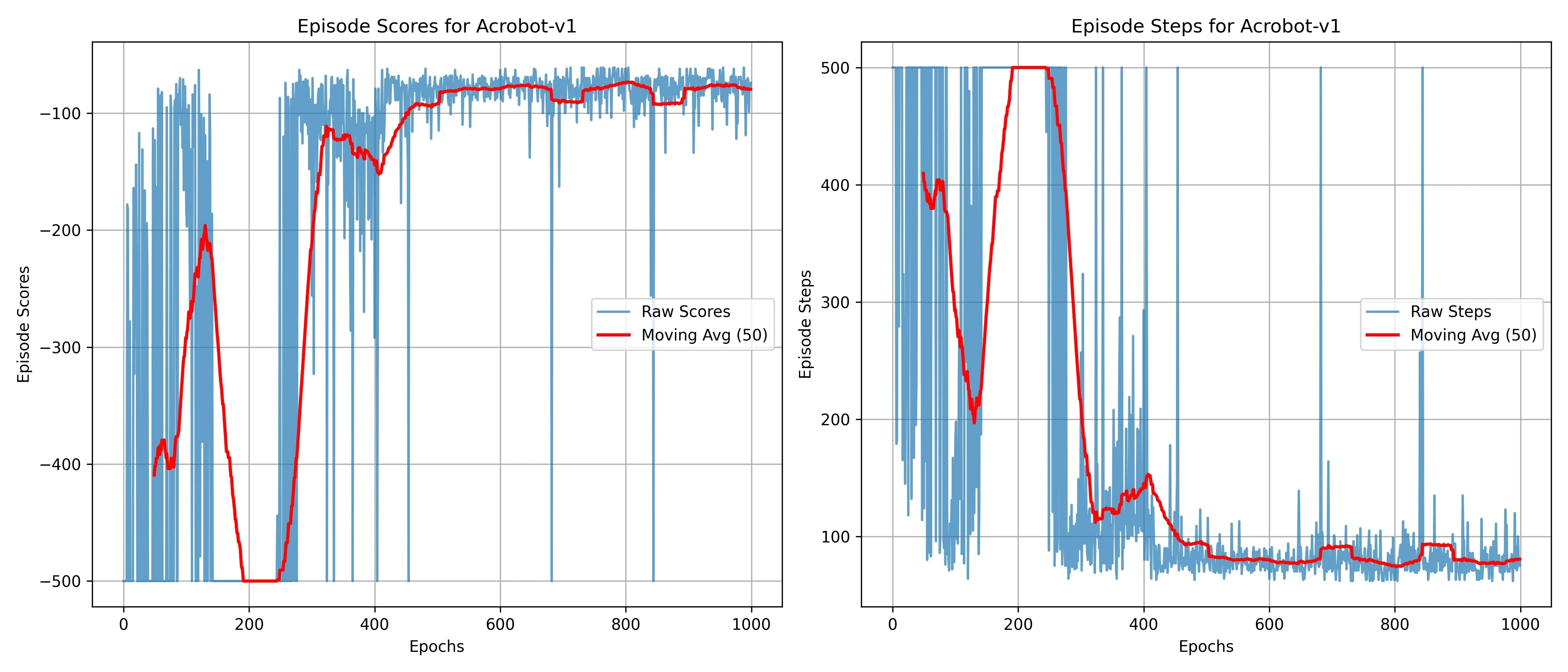
Figure 31 shows the expected pattern of rapid improvement within 200 epochs, with efficient episode completion maintained throughout training. The excellent score stability in Figure 32 (standard deviation: 13.76) confirms PER's ability to improve an already-successful algorithm without hurting its core performance.
MountainCar-v0 Results
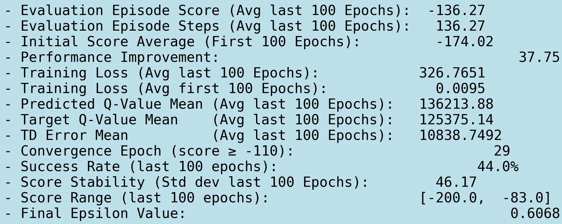
On MountainCar-v0, PER improved on Double DQN but failed to overcome the fundamental sparse-reward pathology. It reached a 44% success rate with a final score of -136.27, close to vanilla DQN (46%).
Figure 33 shows early convergence at epoch 29, but overall progress is limited. Prioritized sampling helps identify and reuse rare successful experiences, but it does not solve the fundamental problem: successful experiences themselves are too rare.
In MountainCar, when the agent reaches the goal by chance, that experience has a high TD error and is sampled repeatedly by PER. But a single successful trajectory is not enough to learn a generalized "swing" strategy. Successful experiences from a variety of initial conditions are needed, and collecting them is itself the challenge of a sparse-reward environment.
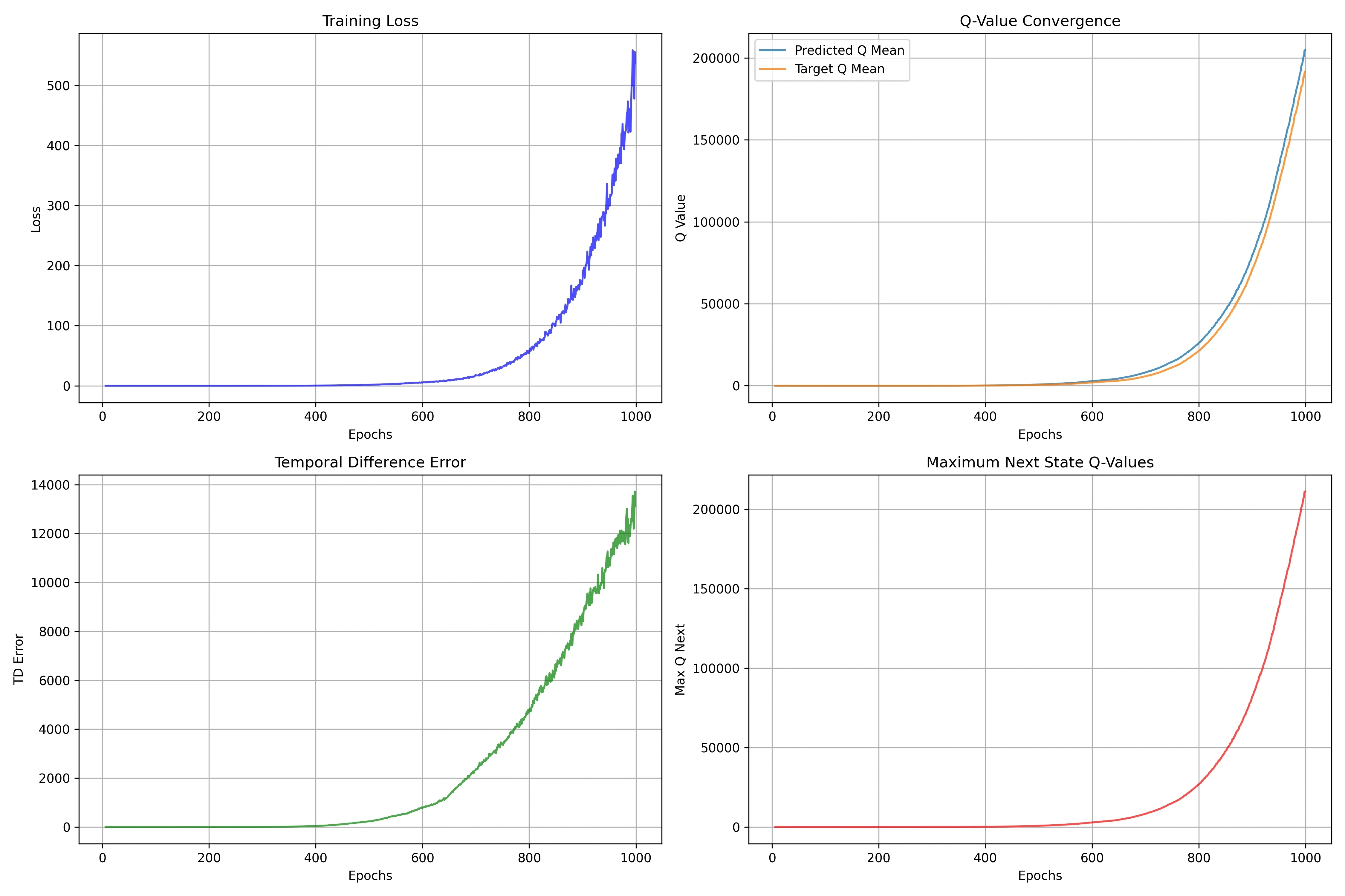
Figure 34 shows worrying training instability with extremely high Q-values (>100,000) and massive TD errors (>10,000). This exposes a limitation of PER: in sparse-reward settings, repeatedly learning from rare successful experiences can cause Q-values to explode.
When rare successful experiences receive extremely high priority and are sampled repeatedly, the Q-values become unrealistically high, and these high Q-values in turn inflate the TD errors, creating a vicious cycle. Tuning the α parameter can mitigate this, but it is not a fundamental fix.
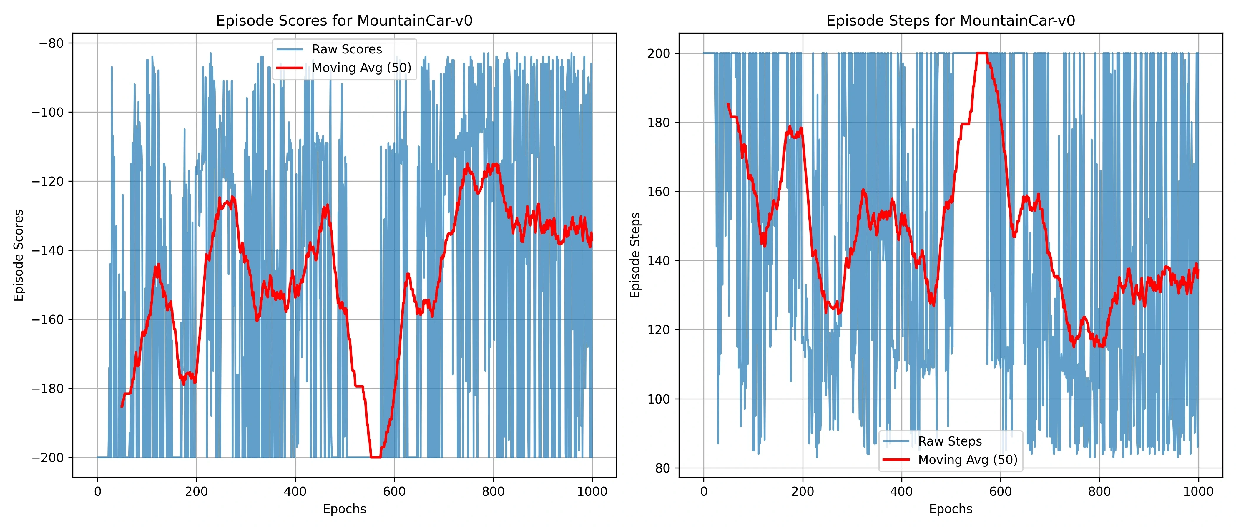
Figure 35 shows an erratic performance pattern similar to the earlier algorithms, confirming that the fundamental exploration-exploitation challenge was not solved. The metrics in Figure 36 show that while PER can identify important transitions, it cannot generate the structured exploration needed for a consistent momentum-building strategy in MountainCar.
Overall PER Analysis
The PER implementation offers valuable insight into the relationship between experience replay strategies and environment characteristics.
On CartPole-v1, PER achieved the best performance of all tested algorithms (51.3% of optimal vs. 43.9% for Double DQN and 35.6% for vanilla DQN), validating the theoretical advantage of prioritized sampling in environments where critical transitions are rare but learnable. The improved success rate (38% vs. 27% for Double DQN) confirms that focusing on high-error transitions can greatly improve learning efficiency in environments with scarce successful experiences.
The Acrobot-v1 results confirm PER's ability to improve an already-successful algorithm without introducing instability, keeping a 93% success rate while improving score consistency.
However, MountainCar-v0 exposes PER's limits in truly sparse-reward environments, where amplifying large prediction errors can destabilize training rather than improve learning. The extreme Q-value inflation and training instability confirm that prioritized sampling needs careful tuning and can be counterproductive when combined with an environment that provides insufficient learning signal density.
6. Overall Results and Analysis
Performance Comparison
| Environment | Metric | DQN | Double DQN | PER |
|---|---|---|---|---|
| CartPole-v1 | Success rate | 12% | 27% (+125%) | 38% (+217%) |
| Average score | 178.13 | 219.38 | 256.73 | |
| Std. dev. | 148.55 | 181.27 | 200.18 | |
| Acrobot-v1 | Success rate | 99% | 95% | 93% |
| Average score | -76.41 | -75.98 | -77.89 | |
| Std. dev. | 43.5 | 12.11 | 13.76 | |
| MountainCar-v0 | Success rate | 46% | 21% | 44% |
| Average score | -114.21 | -143.14 | -136.27 |
Key Findings
1. Environment Characteristics Determine Algorithm Performance
The most important finding is that the reward structure, not the complexity of the state space, determines algorithm performance.
- Acrobot (6-dimensional): DQN 99% success - complex, but dense reward
- MountainCar (2-dimensional): DQN 46% success - simple, but sparse reward
This suggests that analyzing the environment's reward structure should come first when choosing an algorithm. Rather than expecting the performance reported in papers, you should first understand the characteristics of your own problem environment.
2. Fixing Q-Value Overestimation Alone Is Not Enough
On CartPole, Double DQN reduced overestimation to 0, but the success rate was only 27%. This confirms that policy fragility has many causes, and overestimation is just one of them.
Other potential causes:
- High variance in policy gradients
- Limited network capacity
- Poor exploration-exploitation balance
3. Conservative Value Estimation Is a Double-Edged Sword
On MountainCar, Double DQN actually performed worse than DQN (21% vs. 46%). This is a counterintuitive result.
Mechanism: in a sparse-reward environment, the agent receives a meaningful learning signal only when it reaches the goal by chance. DQN's optimistic Q-value estimates provide an incentive that says "worth a try," which encourages exploration. Double DQN's conservative estimates suppress this incentive to explore.
Implication: algorithm modifications must match the environment's requirements. Sparse-reward environments may need optimistic exploration.
4. PER Is an Incremental Improvement, Not a Fundamental Solution
It achieved the best performance on CartPole (38%), but it did not solve MountainCar's fundamental problem.
PER's premise: important experiences must exist in the buffer and be identifiable by their TD errors.
MountainCar's problem: successful experiences are so rare that PER has nothing to prioritize.
Sparse-reward environments need more fundamental solutions, such as intrinsic motivation (curiosity-driven learning), hierarchical RL, or model-based approaches.
5. Environment Analysis Should Come Before Algorithm Selection
How well the environment's reward structure matches the algorithm's assumptions matters more than theoretical superiority.
Practical guidelines:
- Dense-reward environments: DQN is enough; Double DQN/PER improve stability
- Sparse-reward environments: recognize the limits of DQN-based methods and look for alternatives
- In-between environments (CartPole): improvement in the order PER > Double DQN > DQN
7. Conclusion and Future Work
Project Conclusion
Through this project, I implemented and experimented with three algorithms, DQN, Double DQN, and PER, and confirmed their characteristics and limits firsthand.
Main Findings
-
DQN performs excellently in a dense-reward environment (Acrobot), but is unstable in some environments because of overestimation bias
-
Double DQN effectively solves the overestimation problem, but can actually perform worse in sparse-reward environments
-
PER improves learning efficiency by focusing on important transitions, but does not solve the fundamental problem of sparse rewards
-
Contrary to the common belief that "Double DQN is always better than DQN," experiments confirmed that it can backfire depending on the environment
-
Analyzing the environment's reward structure should come first when choosing an algorithm
What I Learned
Reading a paper and understanding an algorithm is a different experience from implementing it yourself. During implementation, I felt firsthand the importance of detailed decisions that papers do not cover (hyperparameters, numerical stability, per-environment tuning).
Future Work
1. Improving Sparse-Reward Environments
Methods for solving the sparse reward problem identified in MountainCar:
Intrinsic Motivation (Curiosity-Driven Learning)
- Give an intrinsic reward for "exploring new states" itself, in addition to the external reward
- ICM (Intrinsic Curiosity Module), RND (Random Network Distillation), etc.
Reward Shaping
- Design intermediate rewards based on distance to the goal, velocity, and so on
- Caution: bad shaping can lead to a solution for a different problem than the original
Hierarchical RL
- Separate high-level goals ("climb the left hill") from low-level actions ("accelerate")
- Option framework, Feudal Networks, etc.
2. Extending the Algorithms
Dueling DQN
- Decompose into Q(s,a) = V(s) + A(s,a)
- Learn the state value and the action advantage separately
Noisy DQN
- Add noise to the network parameters instead of using ε-greedy
- Exploration in parameter space
Distributional RL (C51, QR-DQN)
- Learn the full distribution of Q-values instead of their expected value
- Use the uncertainty information
3. Applying to Real Problems
Applying the implemented algorithms to more complex environments:
- Atari games: reproduce the original paper's benchmarks
- Robot control: extend to continuous action spaces (DDPG, SAC)
- Multi-agent: cooperative/competitive environments
References
-
Mnih, V., Kavukcuoglu, K., Silver, D., Rusu, A. A., Veness, J., Bellemare, M. G., ... & Hassabis, D. (2015). "Human-level control through deep reinforcement learning." Nature, 518(7540), 529-533.
-
van Hasselt, H., Guez, A., & Silver, D. (2016). "Deep Reinforcement Learning with Double Q-learning." Proceedings of the AAAI Conference on Artificial Intelligence, 30(1).
-
Schaul, T., Quan, J., Antonoglou, I., & Silver, D. (2016). "Prioritized Experience Replay." International Conference on Learning Representations (ICLR).
-
Wang, Z., Schaul, T., Hessel, M., Hasselt, H., Lanctot, M., & Freitas, N. (2016). "Dueling Network Architectures for Deep Reinforcement Learning." International Conference on Machine Learning (ICML).
-
Sutton, R. S., & Barto, A. G. (2018). "Reinforcement Learning: An Introduction (2nd ed.)." MIT Press.
-
OpenAI Gymnasium Documentation: https://gymnasium.farama.org/
Appendix: Code Repository
The full implementation is organized as a Jupyter Notebook. It includes each algorithm's hyperparameters, instructions for reproducing the experiments, and the result visualization code.