The 3 key points of this post
- Gradient descent needs the slope (gradient) of every weight. Nudging the weights one at a time and measuring would take 200,000 forward passes for 100,000 weights, but backpropagation gets them all with one forward pass plus one pass of similar cost.
- Backpropagation applies the chain rule of differentiation backward, starting from the loss. Each operation only has to "multiply the gradient it receives by its own derivative and pass it on."
- Writing a 784-128-10 network by hand in NumPy and training it on handwritten digits (MNIST) reaches 97.7% test accuracy in 1.6 seconds on a Mac M1 Max CPU.
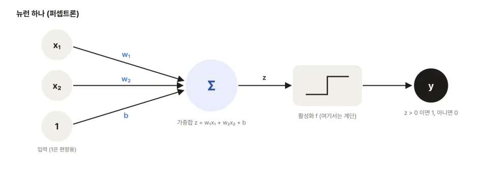
This is the second post in the AI Note series. In Part 1, we said a neural network is a function built by stacking neurons in layers, and training is reducing the loss with gradient descent. But to do gradient descent, we need to know, for every weight, "how much does the loss change if I change this weight a little," that is, the gradient . This post walks step by step through backpropagation, the efficient way to compute it, starting from small numeric examples, then implements it and trains on real data.
1. Why We Need Backpropagation
The simplest approach is to nudge each weight by a tiny amount (numerical differentiation).
This is accurate but expensive. The network we build in this post has 101,770 weights. Each weight needs the loss computed twice, so taking a single step requires about 200,000 forward passes. Backpropagation gets the same result with 1 forward pass and 1 backward pass of similar cost. That is a 100,000x difference. Without backpropagation, deep learning as we know it would not be possible.
2. Starting Point: The Chain Rule
Backpropagation is not new math. It is a systematic way to use the chain rule taught in high school. When functions are nested, the derivative is the product of the derivatives of each step.
For example, let's differentiate at . Let , so .
| Step | Value () | Local derivative |
|---|---|---|
| Chain rule |
Expanding to check: , , the same. There are two important observations here. First, each step only needs to know the derivative of its own operation (the local derivative). Second, computing requires from the forward pass. These two points are all there is to backpropagation.
3. Viewing It as a Computational Graph
Breaking an expression into individual operations connected by arrows gives a computational graph. Let's compute at .
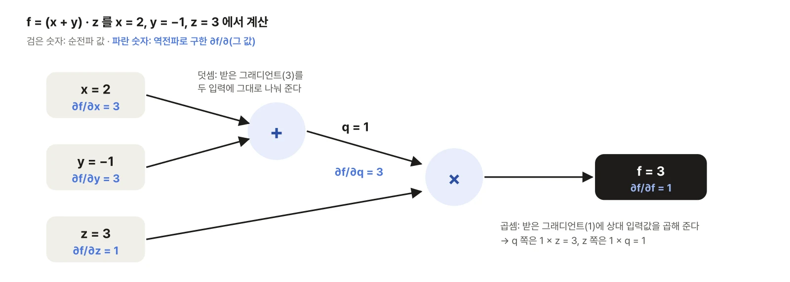
- Forward pass (left → right): , .
- Backward pass (right → left): the starting point is .
- Multiplication : , . Multiplication passes on the received gradient times the other input's value.
- Addition : since , it passes the received gradient 3 unchanged to both inputs. So .
Check: changing from 2 to 2.01 gives , an increase of 0.03. A change of 0.01 yields 0.03, so the slope of 3 is correct.
Remember the rules from this example and any complicated expression can be solved the same way.
| Operation | What it does in the backward pass |
|---|---|
| Addition | Passes the received gradient unchanged to every input |
| Multiplication | Multiplies the received gradient by the other input's value |
| ReLU | Passes it through if in the forward pass, otherwise 0 |
| Same value used in several places | Adds up the gradients returning from each path |
4. One Training Step with a Single Neuron
Now let's train a real neuron for one step. Input , weight , bias , ReLU activation, target , and squared-error loss .
Forward pass
| Step | Computation | Value |
|---|---|---|
| Weighted sum | 1.5 | |
| Activation | 1.5 | |
| Loss | 2.25 |
Backward pass (backward from the loss)
| Gradient | Computation | Value |
|---|---|---|
| −3 | ||
| (passes through ReLU since ) | −3 | |
| (multiplication: multiply by the other input ) | −6 | |
| (addition: unchanged) | −3 |
Update (learning rate ): , .
Running the forward pass again gives and . We reached the target in one step (the numbers in this example were chosen to work out exactly; in practice it takes thousands of steps). A negative gradient means "increasing reduces the loss," which is why gradient descent increased .
5. A Whole Layer: Writing It with Matrices
A real network handles hundreds of neurons at once, so the same computation is written with matrices. A handwritten digit (MNIST) is a 28×28 = 784-pixel image, and a network with 128 hidden units and 10 outputs (digits 0–9) looks like this. is the number of samples fed in at once (the batch size).
| Value | Shape | Meaning |
|---|---|---|
| Input images | ||
| First-layer weights | ||
| Hidden-layer output | ||
| Second-layer weights | ||
| Per-digit scores and probabilities |
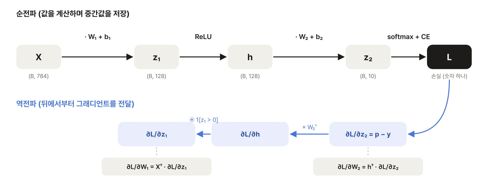
Backpropagation goes backward from the loss, exactly as in section 4.
① Softmax + cross-entropy. Combining the two functions from Part 1 and differentiating gives something surprisingly simple. For one sample, and , so . Differentiating with respect to gives
That is, the probabilities with 1 subtracted from the correct class only. For the example in Part 1 (probabilities 0.659, 0.242, 0.099, correct class 0), the gradient is . It is a signal to raise the correct score and lower the rest. Since we use the batch average, we divide by .
② Second layer. is a multiplication and an addition. Following the rules from section 3, the gradient of multiplies by the other input , and the gradient of multiplies by the other input .
If you are unsure where the transpose () goes, just match the shapes. must have the same shape as , . The only ingredients are and , so , that is, , is the only option. This product automatically sums the gradients from each of the samples in the batch.
③ ReLU. Entries that were negative in the forward pass were blocked at 0, so their gradient is 0 too ( is element-wise multiplication).
④ First layer. Same form as ②. We do not need the gradient of the input , so we skip it.
, , and used in backpropagation are all values computed in the forward pass. It is the same as needing for in section 2. So during training, the forward pass's intermediate values have to stay in memory until backpropagation finishes. That is why training uses much more memory than inference alone.
6. Implementing It from Scratch in NumPy
I translated the equations from section 5 directly into code. No framework like PyTorch, just NumPy.
import numpy as np

def forward(p, X):
    z1 = X @ p['W1'] + p['b1']          # (B,128)
    h = np.maximum(z1, 0)               # ReLU
    z2 = h @ p['W2'] + p['b2']          # (B,10) scores
    z2 = z2 - z2.max(1, keepdims=True)  # subtract the largest score so exp doesn't overflow (same result)
    prob = np.exp(z2) / np.exp(z2).sum(1, keepdims=True)
    return prob, (X, z1, h)             # keep intermediate values for backprop

def backward(p, prob, cache, y):
    X, z1, h = cache
    B = len(y)
    dz2 = prob.copy(); dz2[np.arange(B), y] -= 1; dz2 /= B   # ① subtract 1 from the correct class only
    g = {'W2': h.T @ dz2, 'b2': dz2.sum(0)}                   # ② second layer
    dh = dz2 @ p['W2'].T
    dz1 = dh * (z1 > 0)                                       # ③ ReLU: entries that were negative get 0
    g['W1'] = X.T @ dz1; g['b1'] = dz1.sum(0)                 # ④ first layer
    return g

# minibatch gradient descent: batch 64, learning rate 0.1, 10 epochs (batch splitting abbreviated)
for epoch in range(10):
    for idx in batches(len(X_train), 64):
        prob, cache = forward(p, X_train[idx])
        for k, v in backward(p, prob, cache, y_train[idx]).items():
            p[k] -= 0.1 * v
The bias gradient is .sum(0) because of the last rule in section 3. The same bias was added to every sample in the batch (used in several places), so we sum the gradients returning from each sample. The weights start from He initialization (); why we start this way is covered in the next post. The full code (including data loading and measurement) is about 70 lines.
Verifying the Backpropagation First
Backprop code still trains "to some degree" even when it is wrong, so bugs are easy to miss. That is why we use the numerical differentiation from section 1 as a check. On a small model (20-8-3, batch 5), comparing numerical and backprop gradients for every weight gave a largest relative error of . That means the two are effectively identical. Only after this check did I run training.
Training Results
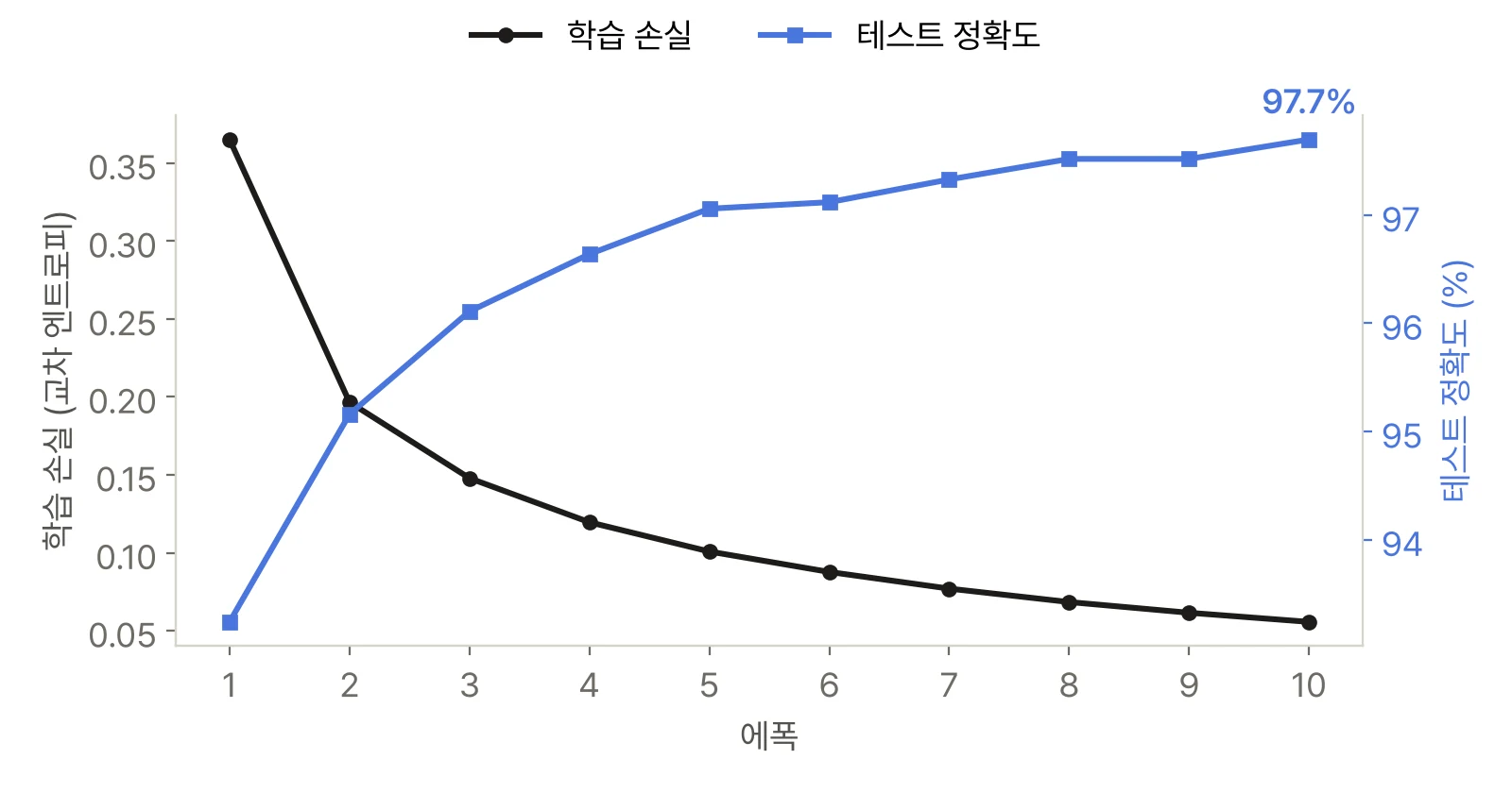
| Epoch | 1 | 2 | 5 | 10 |
|---|---|---|---|---|
| Training loss | 0.365 | 0.197 | 0.101 | 0.056 |
| Test accuracy | 93.2% | 95.2% | 97.1% | 97.7% |
Ten passes over the 60,000 training images took 1.6 seconds in total (including test evaluation after each epoch, about 0.16 seconds per epoch). The hardware is the CPU of a MacBook Pro M1 Max (NumPy 2.5). Accuracy already passes 93% after the first epoch, and after that the loss falls slowly while accuracy creeps up. The model got 9,770 of the 10,000 test images, which were not used for training, right. A network with one hidden layer stalls around 98%, and what breaks through that wall is the CNN, covered from Part 4 onward.
7. Why Train on Minibatches Instead of One Image at a Time
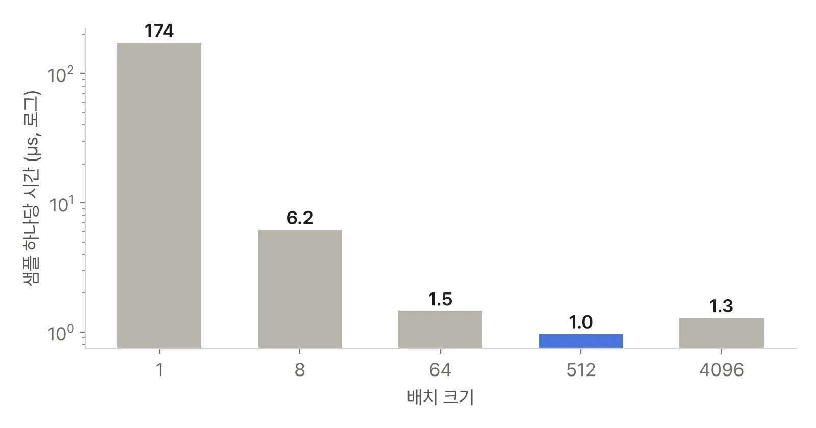
In Part 1, we said the data is grouped into batches of 64 and each batch takes one step (minibatches). There are two reasons for grouping. One is gradient quality. The gradient from a single image swings around depending on that one image, while the average over several images is closer to the direction of the whole dataset. The other is speed. Using the same code and changing only the batch size, I measured the time to process (forward + backward) one sample.
| Batch size | 1 | 8 | 64 | 512 | 4096 |
|---|---|---|---|---|---|
| Time per sample | 174µs | 6.2µs | 1.5µs | 1.0µs | 1.3µs |
The amount of computation per sample is identical (about 410,000 multiply-adds), yet there is a 180x difference between batch 1 and 512. The reason lies in the matrix multiplication from section 5. With a batch of 1, the entire 407 KB weight matrix is read from memory, used for one sample, and discarded. With a batch of 512, the weights read once are reused for 512 samples. For a computer, fetching data is more expensive than computing, so the more times fetched data is reused, the faster it gets. Batch 4096 gets slightly slower again, probably because the input alone grows to 12.8 MB and no longer fits in the CPU cache (a guess).
That said, making the batch arbitrarily large reduces the number of steps per epoch, which can actually slow down training, and it uses more memory too. So in practice the batch size is chosen somewhere between tens and thousands. GPUs are devices specialized for processing large matrix multiplications like this all at once, so the gap becomes much larger with big batches.
8. Summary
- Backpropagation applies the chain rule backward from the loss to get the gradients of all weights for about the cost of one forward pass. It is 100,000x cheaper than numerical differentiation.
- Each operation only needs its local rule. Addition passes the gradient through unchanged, multiplication multiplies by the other input's value, and ReLU passes only the entries that passed in the forward pass.
- The gradient of softmax + cross-entropy is "probabilities − target (one-hot)." Where the transpose goes in a matrix gradient falls out automatically from matching shapes.
- Backpropagation reuses the forward pass's intermediate values. That is why training uses more memory than inference.
- A hand-built two-layer network reaches 97.7% on MNIST. Verify backprop code against numerical differentiation first.
Next post: This time I used He initialization and a learning rate of 0.1 without much explanation. Part 3 compares, with the same kind of hands-on experiments, what happens when initialization goes wrong, and how optimizers such as SGD, Momentum, and Adam, along with normalization, change training.
References
- D. E. Rumelhart, G. E. Hinton, R. J. Williams, "Learning representations by back-propagating errors", Nature 323, 1986.
- K. He et al., "Delving Deep into Rectifiers", ICCV 2015 (He initialization).
- I. Goodfellow, Y. Bengio, A. Courville, Deep Learning, Section 6.5 "Back-Propagation and Other Differentiation Algorithms", MIT Press, 2016.
- Stanford CS231n, "Backpropagation, Intuitions" (backpropagation through computational graphs).
- Y. LeCun, C. Cortes, C. J. C. Burges, The MNIST database of handwritten digits.