Introduction
As part of a CAD algorithms for digital systems course (EE58401), I designed and implemented an algorithm that solves the Rectilinear Steiner Minimum Tree (RSMT) problem. RSMT plays a central role in VLSI (Very Large Scale Integration) design: the goal is to find routing paths that connect a given set of points at minimum cost.
In VLSI chip design, efficiently connecting millions of gates and transistors directly affects the chip's performance, power consumption, and area. Longer wires mean more signal delay, more power consumption, and a larger physical chip area. Finding minimum-length routing, the RSMT problem, is therefore a very important optimization problem in industry.
As semiconductor technology scales down, routing optimization matters even more. In modern semiconductor processes, wire delay often exceeds gate delay, so routing optimization has become a key factor in overall chip performance. At 3nm and 2nm in particular, wire resistance and capacitance increase, which makes optimal routing even more important.
This report implements an RSMT search algorithm based on Dijkstra's algorithm and explains how it handles various problem cases (crossing edges, diagonal edges, loops). It also covers in detail how the quality of the solution is improved through a probabilistic Steiner point selection strategy based on the exponential distribution and through iterative optimization.
Project Overview
The goal of this project is to implement an efficient algorithm that finds an RSMT for a given set of points. The input is a text file in which each line contains x and y coordinates separated by a space. The output is a file containing the coordinates of the edges that make up the RSMT.
Requirements considered when designing the algorithm:
- Correctness: it must produce a valid tree that connects every terminal point.
- Efficiency: it must output a result within the time limit (60 minutes).
- Quality: it should achieve as short a total wirelength as possible.
- Scalability: it must handle inputs of various sizes (3 to 100 points).
I chose Python as the implementation language. Python's strengths are fast prototyping, a rich set of libraries (heapq, random, tqdm, etc.), and readable code. Its weakness, execution speed, was offset by algorithmic optimization and repeated search.
Theoretical Background of the RSMT Problem
What Is the Steiner Tree Problem?
The Steiner tree problem is one of the most important combinatorial optimization problems in graph theory, named after the Swiss mathematician Jakob Steiner (1836). Its goal is to find a minimum-cost tree that connects a given set of vertices (terminals).
The key difference from an ordinary minimum spanning tree (MST) is that additional vertices (Steiner points) may be used. An MST builds the tree from the given vertices only, while a Steiner tree can add new vertices as needed to reduce the total cost.
For example, suppose three points A, B, and C form an equilateral triangle. Connecting them with an MST takes two edges, and the total length is the sum of two sides of the triangle. If each side has length 1, the MST's total length is 2. But adding a Steiner point at the triangle's Fermat point lets all three points connect to that center, cutting the total wirelength to about 1.732 (√3). That is a cost reduction of about 13.4%.
The Steiner tree problem was proven NP-hard by Karp in 1972. This means finding the optimal solution becomes computationally very hard as the input grows. No algorithm is known that guarantees the optimal solution in polynomial time, so practical applications use heuristics or approximation algorithms.
Mathematical Properties of Steiner Points
Steiner points have several important mathematical properties:
-
Degree constraint: in a Euclidean Steiner tree, every Steiner point has degree exactly 3. This is because a point where three edges meet at 120-degree angles is the most energetically stable. In an RSMT, the rectilinear constraint allows degree 2, 3, or 4.
-
Upper bound on the number of Steiner points: with n terminal points, an optimal Steiner tree needs at most n-2 Steiner points. This is easy to prove by induction.
-
Local optimality: a Steiner point sits at the equilibrium of the "forces" from all the terminals connected to it. This can be demonstrated physically with a soap film experiment.
-
Steiner ratio: the ratio of the Steiner tree length to the MST length is called the Steiner ratio. In the Euclidean plane, its lower bound is √3/2 ≈ 0.866, so at most a 13.4% cost reduction is possible. For RSMT, the lower bound of the Steiner ratio is 2/3 ≈ 0.667, allowing up to a 33.3% reduction.
A good way to visualize a Steiner tree is the soap film experiment. Put pins between two glass plates and dip them in soapy water, and the soap film naturally forms the minimum-energy structure connecting the pins. That structure approximates a Steiner tree. For RSMT, running the experiment in a grid-shaped frame lets you observe the rectilinear property.
Rectilinear Steiner Minimum Tree (RSMT)
RSMT is a special form of the Steiner tree problem with two key constraints:
- Manhattan distance: Manhattan distance (the L1 norm) is used instead of Euclidean distance.
- Rectilinear routing: every edge must run only horizontally or vertically.
Manhattan distance is defined as:
These constraints reflect the reality of VLSI design: on a silicon chip, wires are generally laid out only horizontally or vertically. This comes from the limits of the manufacturing process and from design rules that optimize routing density. Technologies supporting 45-degree routing (X-architecture) or other angles have been developing recently, but rectilinear routing is still the most common.
The Hanan Grid Theorem
One of the most important theoretical results for the RSMT problem is the Hanan grid theorem. Proven by Maurice Hanan in 1966, it states that every Steiner point in an optimal RSMT lies on the grid formed by intersecting the x and y coordinates of the terminal points.
Specifically, given n terminal points , the Hanan grid is defined as:
This grid has at most points, but only some of them are Steiner points needed to build the optimal RSMT.
The significance of the Hanan grid theorem is that it shrinks the search space from an infinite continuous space to a finite discrete one. Even so, finding the right combination among candidate points remains NP-hard.
Approximation Ratios for RSMT
Approximation algorithms for RSMT are also an active research area. The simplest approximation uses the MST, which gives an approximation ratio of 2. In other words, an MST-based solution is guaranteed to be within 2 times the optimum.
More sophisticated algorithms achieve better approximation ratios:
- 1-Steiner algorithm: approximation ratio of about 1.5
- Iterated 1-Steiner algorithm: approximation ratio of about 1.3
- PTAS (Polynomial Time Approximation Scheme): theoretically allows a approximation
Applications of RSMT
RSMT plays a key role in many fields:
-
VLSI physical design: optimizing the routing paths that connect gates, flip-flops, memory cells, and so on inside a chip. Modern processors have billions of transistors, and the efficiency of the wiring that connects them determines chip performance.
-
PCB design: optimizing connections between components on a printed circuit board. Minimizing the routing on each layer of a multilayer PCB improves manufacturing cost and signal integrity.
-
Communication networks: optimizing cable placement between nodes. Minimizing physical cable length in data centers and telecom networks reduces cost and latency.
-
Architecture and urban planning: designing pipe or wire routes. Used for plumbing systems in buildings and for city power grid design.
-
Multi-chip modules (MCM): routing optimization in the design of interposers that connect multiple dies.
-
FPGA routing: optimizing connections between logic blocks in a field programmable gate array. FPGA routing resources are limited, so efficient routing matters.
-
Clock tree synthesis (CTS): designing the tree that distributes the clock signal to flip-flops. The goal is to minimize total wirelength along with skew.
Where RSMT Fits in the VLSI Design Flow
RSMT is used in the physical design stage of the VLSI design flow. The overall flow looks like this:
- RTL design: functional design in Verilog/VHDL
- Synthesis: converting RTL to gate level
- Floorplanning: block placement
- Placement: cell placement
- Global routing: deciding rough paths with RSMT
- Detailed routing: finalizing the actual wire paths
- Timing analysis and optimization: performance verification
RSMT is used mainly in the global routing stage. The RSMT produced there guides detailed routing and has a large impact on the quality of the final routing.
Algorithm Design
Overall Algorithm Flow
The RSMT algorithm I designed consists of the following steps:
- Data parsing: read point coordinates from the input file
- Steiner point candidate computation: generate candidates from the Hanan grid
- Steiner point selection: probabilistic selection using the exponential distribution
- RSMT search: build the tree based on Dijkstra's algorithm
- Problem case handling: remove crossing edges, diagonal edges, and loops
- Optimization: remove unnecessary Steiner points
- Iterative optimization: repeat the search within the time limit
I concretely implemented the problem cases that can arise at each step and how to resolve them. In particular, I designed logic that systematically handles crossings, diagonal connections, and loops, which come up often in real routing problems.
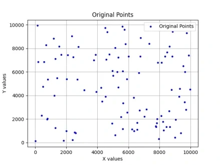
The figure above shows the distribution of the original points given as input. 100 points are spread over a 10000×10000 two-dimensional space, and the goal is to connect them with a minimum-length rectilinear tree. The points are fairly evenly distributed, but some areas are dense, which shows why efficient Steiner point placement matters.
Point Class Design
I defined a Point class as the algorithm's basic data structure:
class Point:
    def __init__(self, x, y):
        self.x = x
        self.y = y

    def __str__(self):
        return f"{self.x:4d} {self.y:4d}"
It is a simple structure, but it is useful for managing 2D coordinates efficiently and keeping the output format consistent. Coordinates are handled as integers to avoid floating-point errors. The output uses a fixed width of 4 digits to make log files easier to read.
Parsing the Input Data
I implemented a function that reads point coordinates from the input file:
def parse_points_from_file(filename):
    points = []
    try:
        with open(filename, 'r') as file:
            for line in file:
                x, y = map(int, line.split())
                point = Point(x, y)
                points.append(point)
    except FileNotFoundError:
        print(f"Error: The file '{filename}' was not found.")
    except Exception as e:
        print(f"An error occurred: {e}")
    return points
Exception handling lets the program exit safely even when the file is missing or malformed. The input format is assumed to be a simple text file with x and y coordinates separated by a space on each line.
Generating Steiner Point Candidates
All possible Steiner point candidates are generated from the Hanan grid:
def find_all_points(points):
    all_points = []

    x_coords = sorted(set(p.x for p in points))
    y_coords = sorted(set(p.y for p in points))

    for x in x_coords:
        for y in y_coords:
            all_points.append(Point(x, y))

    return all_points
This function works as follows:
- Extract the x coordinates of all original points, remove duplicates, and sort them
- Extract the y coordinates of all original points, remove duplicates, and sort them
- Generate every (x, y) combination to build the Hanan grid
With n original points, up to n² grid points are generated. For example, 100 points can generate up to 10,000 grid points. The ones other than the original points become Steiner point candidates.
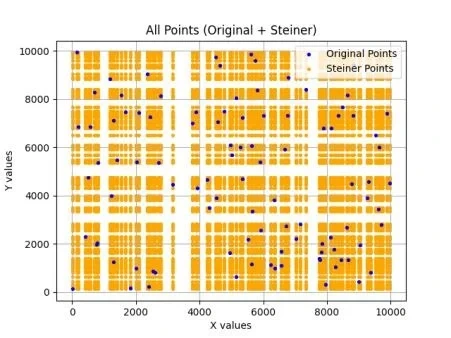
The figure above shows all the Steiner point candidates (orange) generated from the Hanan grid. Every point where the x and y coordinates of the blue original points intersect becomes a candidate, forming a grid. The density of this grid gives a sense of how large the search space is.
Computing Manhattan Distance
A function that computes the Manhattan distance between two points:
def manhattan_distance(p1, p2):
    return abs(p1.x - p2.x) + abs(p1.y - p2.y)
RSMT uses Manhattan distance rather than Euclidean distance. Manhattan distance is also called "taxicab distance": it equals the distance a taxi travels in a city laid out on a grid. Since VLSI allows only rectilinear routing, this metric is appropriate.
Properties of Manhattan distance:
- It is always greater than or equal to the Euclidean distance (equal only for horizontal/vertical moves)
- It is simple and fast to compute (no square root needed)
- It returns exact integer results for integer coordinates
Analyzing the relationship mathematically, the Manhattan distance between two points is between 1 and √2 times the Euclidean distance. Specifically, the two distances are equal when the points are aligned horizontally or vertically, and the Manhattan distance is √2 times the Euclidean distance when they lie at a 45-degree angle. This difference also affects the ratio between the optimal RSMT and the optimal Euclidean Steiner tree.
The reason VLSI design uses Manhattan distance has to do with physical constraints. In chip manufacturing, wires are formed on specific metal layers, and each layer has a preferred direction. For example, it is common for M1 to route horizontally and M2 vertically. Because of these constraints, diagonal routing is physically impossible or inefficient, so Manhattan distance accurately reflects actual wirelength.
Computing Total Wirelength
To evaluate the quality of the final RSMT, I implemented a function that computes the total wirelength:
def calculate_total_length(all_points, rmst_edges):
    total_length = 0
    for u, v in rmst_edges:
        if all_points[u] is not None and all_points[v] is not None:
            total_length += manhattan_distance(all_points[u], all_points[v])
    return total_length
This function sums the Manhattan distance over every edge of the tree. Removed points, marked as None, are skipped. The total length serves as both the algorithm's optimization objective and its performance metric.
Exponential-Distribution-Based Steiner Point Selection
Using every candidate Steiner point would make the computational complexity too high. Considering all of the up to 10,000 candidates generated from 100 terminals makes it hard to find a solution in time. So I used a strategy of probabilistically selecting only some of them:
LAMBDA = 20

random_val = min(max(int(random.expovariate(LAMBDA) * (len(steiner_points) - 1)), 0), len(steiner_points))
selected_steiner_points = random.sample(steiner_points, random_val)
The reasons for using the exponential distribution are as follows:
-
Preference for few Steiner points: the exponential distribution is likely to produce small values, so it tends to select few Steiner points. This improves computational efficiency.
-
Diversity: it still occasionally selects many Steiner points, leaving open the chance of finding a better solution. The long tail of the exponential distribution makes this possible.
-
Tuning with LAMBDA: the larger LAMBDA is, the stronger the tendency to select few Steiner points. LAMBDA = 20 was chosen experimentally to balance computation time and solution quality.
-
Memorylessness: thanks to the memoryless property of the exponential distribution, each iteration makes an independent selection.
The probability density function of the exponential distribution is:
With LAMBDA = 20, the expected value is 1/20 = 0.05, so on average about 5% of all candidates are selected.
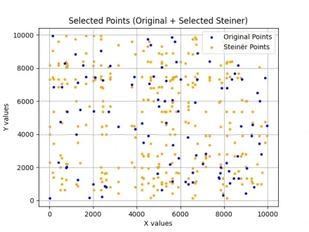
The figure above shows the Steiner points selected probabilistically through the exponential distribution. Only some of the candidates are selected, which greatly improves computational efficiency. The selected points are spread fairly evenly, so they can contribute to the overall tree structure.
Dijkstra-Based RSMT Search
Algorithm Overview
Dijkstra's algorithm originally finds the shortest paths from a single source to every vertex in a graph. It was devised in 1956 by the Dutch computer scientist Edsger Dijkstra and is considered a classic among graph algorithms.
My RSMT search uses a slightly modified Dijkstra's algorithm to build a minimum spanning tree. Like Prim's algorithm, it uses a priority queue to add the nearest point to the tree one at a time.
The differences from Prim's algorithm are:
- Prim: add the vertex closest to the current tree
- Dijkstra variant: add the vertex with the smallest cumulative distance from the source
In practice, for an RSMT problem using Manhattan distance, the two approaches produce similar results.
def find_rsmt_dijkstra(original_points, selected_steiner_points, all_points):
    num_points = len(all_points)
    dist = [float('inf')] * num_points
    parent = [-1] * num_points
    visited = [False] * num_points
    edges = []

    dist[0] = 0
    queue = [(0, 0)]  # (distance, node)

    while queue:
        _, u = heapq.heappop(queue)
        if visited[u]:
            continue
        visited[u] = True
        if parent[u] != -1:
            edges.append((parent[u], u))
        for v in range(num_points):
            if visited[v] or u == v:
                continue
            w = manhattan_distance(all_points[u], all_points[v])
            if w < dist[v]:
                dist[v] = w
                parent[v] = u
                heapq.heappush(queue, (w, v))
Detailed Analysis of the Algorithm
-
Initialization:
distarray: the current shortest distance to each vertex, initialized to infinityparentarray: the parent node of each vertex (stores the tree structure)visitedarray: visited flags- Set the distance of the start point (node 0) to 0
-
Iteration:
- Pop the node with the smallest distance from the priority queue
- Skip it if already visited
- Mark it visited, and add an edge if it has a parent
- Update distances for all neighboring nodes and push them onto the queue
-
Termination:
- Stop when the queue is empty
- Every connected node is now in the tree
Using a Priority Queue
I implemented a min-heap-based priority queue with Python's heapq module. Properties of a min-heap:
heappush: inserts an element in O(log n) timeheappop: extracts and removes the minimum element in O(log n) time- Heap invariant: a parent node is always less than or equal to its children
This makes it efficient to extract the point with the smallest distance each time. A linear search over an array would take O(n), but a heap reduces it to O(log n).
Understanding how the heap works internally helps in understanding how the algorithm behaves. A heap is represented as a complete binary tree and can be implemented efficiently with an array. For a node at index i, its parent is at (i-1)//2, its left child at 2i+1, and its right child at 2i+2. On heappush, the new element is added at the end of the tree and moves up by comparing with its parent (sift-up). On heappop, the root is removed, the last element moves to the root, and it moves down by comparing with its children (sift-down).
Python's heapq module is implemented in C, so it is considerably faster than a pure Python implementation. However, it does not support some advanced operations (such as decrease-key). If needed, a custom heap or an external library (such as sortedcontainers) can be considered.
Time Complexity Analysis
Let's analyze the algorithm's time complexity step by step:
Step 1: Generating Steiner point candidates - O(n²)
x_coords = sorted(set(p.x for p in points))  # O(n log n)
y_coords = sorted(set(p.y for p in points))  # O(n log n)
for x in x_coords:  # O(n)
    for y in y_coords:  # O(n)
        all_points.append(Point(x, y))  # O(1)
In the worst case, n² grid points are generated.
Step 2: Selecting Steiner points - O(k) k Steiner points are selected via the exponential distribution. random.sample takes O(k) time.
Step 3: Dijkstra search - O(m² log m) Dijkstra runs over m = n + k points. Each point computes the distance to every other point (O(m)) and pushes onto the heap (O(log m)), for a total of O(m² log m).
Step 4: Problem case handling - O(e²) Crossing checks are performed over e edges. In the worst case every pair must be checked, so O(e²). In a tree, e = m - 1, so this is O(m²).
Step 5: Optimization - O(m²) Every edge and point is checked in each iteration.
Overall time complexity: one search is O(m² log m), repeated up to T times, so O(T × m² log m), where T is the number of iterations and m is the total number of points.
Space complexity: the O(m²) distance information is not stored but computed on demand, so the space complexity is O(m), storing only point and edge information.
The following optimizations are possible for a more efficient implementation:
- Use an implicit graph instead of adjacency lists (the current implementation)
- Nearest-neighbor search with a k-d tree - O(log n) nearest-neighbor queries on average
- Accelerate distance computation with parallel processing - use multiple cores
- Precomputed tables (the FLUTE approach) - O(1) lookup for small problems
Handling Problem Cases
After building the initial tree with Dijkstra's algorithm, three main problem cases must be handled. They must be resolved to satisfy the RSMT constraints (rectilinear routing, no cycles).
1. Handling Crossing Edges
Two edges must not cross in an RSMT, because:
- Routing integrity: in real VLSI, two wires crossing on the same layer cause a short circuit
- Tree structure violation: unless the crossing point is made a node, the result is not a tree
A function that detects whether two edges cross:
def is_crossing(p1, p2, p3, p4):
    def direction(a, b, c):
        return (b.x - a.x) * (c.y - a.y) - (b.y - a.y) * (c.x - a.x)

    d1 = direction(p1, p2, p3)
    d2 = direction(p1, p2, p4)
    d3 = direction(p3, p4, p1)
    d4 = direction(p3, p4, p2)

    if p1 == p3 or p1 == p4 or p2 == p3 or p2 == p4:
        return False  # segments that share an endpoint are not treated as crossing

    return (d1 * d2 < 0) and (d3 * d4 < 0)
This function uses the CCW (counter-clockwise) algorithm to decide whether two line segments cross. How the CCW algorithm works:
-
The
direction(a, b, c)function computes the orientation of three points- Positive: counter-clockwise
- Negative: clockwise
- 0: collinear
-
Crossing condition for segments (p1-p2) and (p3-p4):
- p3 and p4 must lie on opposite sides of segment p1-p2
- p1 and p2 must lie on opposite sides of segment p3-p4
-
The crossing is decided from the combination of signs of the orientation values
When a crossing is found, a new Steiner point is added at the intersection and the edges are rebuilt:
if is_crossing(p1, p2, p3, p4):
    # Compute the intersection point
    if p1.x == p2.x:  # first edge is vertical
        mid_point_x = p1.x
        mid_point_y = p3.y
    else:  # second edge is vertical
        mid_point_x = p3.x
        mid_point_y = p1.y

    mid_point = Point(mid_point_x, mid_point_y)
    # Add the new Steiner point and rebuild the edges
In rectilinear routing, when two segments cross, one is horizontal and the other vertical. So the intersection is easily computed from the x coordinate of the vertical segment and the y coordinate of the horizontal one.
After the crossing is resolved, the original two edges are replaced by four. For example, if A-B and C-D meet at intersection X, they are rebuilt as A-X, X-B, C-X, and X-D. This removes the crossing without changing the total wirelength.
The time complexity of the crossing check is O(e²), since every pair of edges must be checked: up to e(e-1)/2 pairs for e edges. A more efficient implementation could use a sweep-line algorithm or spatial partitioning.
2. Handling Diagonal Edges
In an RSMT, every edge must be horizontal or vertical. Dijkstra's algorithm can produce diagonal edges, so they must be handled.
def is_diagonal(p1, p2):
    return p1.x != p2.x and p1.y != p2.y

# Handle diagonal edges
if is_diagonal(all_points[u], all_points[v]):
    edges.pop(l)
    mid_point = Point(all_points[u].x, all_points[v].y)
    all_points.append(mid_point)
    selected_steiner_points.append(mid_point)

    mid_point_index = len(all_points) - 1
    edges.append((u, mid_point_index))
    edges.append((mid_point_index, v))
When a diagonal edge (u, v) is detected:
- Remove the original edge
- Create a midpoint with u's x coordinate and v's y coordinate (the corner of an L)
- Add the midpoint to the Steiner point list
- Replace the edge with two rectilinear edges: (u, mid) + (mid, v)
This turns the original diagonal path into an L-shaped rectilinear path. Because of how Manhattan distance works, the total length stays the same.
There are two options for the direction of the L-shaped path: (1) move horizontally first, then vertically, or (2) move vertically first, then horizontally. The current implementation uses the first, but when congestion or obstacles are considered, the other direction may be better. This can be considered as a future improvement.
3. Detecting and Removing Loops
A tree must not contain cycles. However, the edge rebuilding process can unintentionally create them.
def find_loops(edges):
    loops = []
    edge_dict = {}

    # Convert edges into a dictionary
    for u, v in edges:
        if u not in edge_dict:
            edge_dict[u] = []
        if v not in edge_dict:
            edge_dict[v] = []
        edge_dict[u].append(v)
        edge_dict[v].append(u)

    # Detect loops
    for u in edge_dict:
        if len(edge_dict[u]) >= 2:
            for i in range(len(edge_dict[u])):
                for j in range(i + 1, len(edge_dict[u])):
                    v1, v2 = edge_dict[u][i], edge_dict[u][j]
                    if v1 in edge_dict and v2 in edge_dict:
                        common_neighbors = set(edge_dict[v1]) & set(edge_dict[v2])
                        for cn in common_neighbors:
                            if cn != u and len({u, v1, v2, cn}) == 4:
                                loops.append([(u, v1), (u, v2), (v1, cn), (v2, cn)])

    return loops
This function detects rectangular loops made of four points:
- Convert the edges into adjacency-list form
- At each node, pick two neighbors
- If the two neighbors share a common neighbor, a loop is formed
- Add the detected loop to the list
When a loop is found, one edge is removed at random to keep the tree structure. The random choice avoids bias toward any particular pattern.
A typical case where a rectangular loop forms is when two L-shaped paths share the same start and end points. For example, if there are two paths from point A to point B, A→M1→B and A→M2→B, the four edges (A-M1, M1-B, A-M2, M2-B) form a rectangular loop. Removing one of them breaks the loop and restores the tree structure.
A general cycle detection algorithm (DFS, Union-Find, etc.) could also be used, but since most cycles that arise in RSMT are rectangular, a specialized function is more efficient. Larger cycles (5 or more nodes) are rare and are mostly resolved along with the rectangular loop removal.
Problem case handling is performed repeatedly, because fixing one problem can create another. For example, adding a new Steiner point to resolve a crossing can create diagonal edges or new loops. So the checks repeat until every problem is resolved.
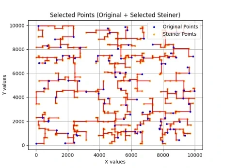
The figure above shows the initial RSMT result after Dijkstra's algorithm and problem case handling. The red lines are the routing paths, and every original point (blue) is connected. The orange points are the Steiner points in use.
Optimization Process
Removing Unnecessary Steiner Points
The initial RSMT may contain unnecessary Steiner points. In particular, Steiner points of degree 1 (points with only one edge attached) can be removed to reduce total length without affecting the tree's connectivity.
Why can degree-1 Steiner points be removed?
- A Steiner point is not a terminal, so it does not have to be connected
- At degree 1, only one edge is attached
- Removing that edge does not affect the connectivity of the other nodes
- Removing it reduces the total length by that edge's length
def remove_single_edge_points(final_edges, all_points, selected_steiner_points):
    is_change = False

    # Count the edges attached to each Steiner point
    edge_count = [0] * len(all_points)

    for u, v in final_edges:
        if all_points[u] and all_points[u] in selected_steiner_points:
            edge_count[u] += 1
        if all_points[v] and all_points[v] in selected_steiner_points:
            edge_count[v] += 1

    # Remove Steiner points of degree 1
    for i, count in enumerate(edge_count):
        if count == 1:
            final_edges = [(u, v) for u, v in final_edges if u != i and v != i]

            index_to_remove = next((index for index, point in enumerate(selected_steiner_points) if
                                    point.x == all_points[i].x and point.y == all_points[i].y), None)
            if index_to_remove is not None:
                selected_steiner_points.pop(index_to_remove)
                all_points[i] = None

            is_change = True

    return all_points, selected_steiner_points, final_edges, is_change
This process repeats until nothing changes, yielding the final RSMT. Repetition is needed because removing one Steiner point can lower another Steiner point's degree, making it a new candidate for removal.
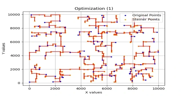
This is an early stage of the optimization process. Unnecessary Steiner points are being removed gradually.
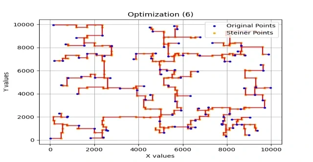
This is the optimization result after 6 steps. The tree structure has become noticeably more compact. Every remaining Steiner point has degree 2 or more and actually contributes to routing efficiency.
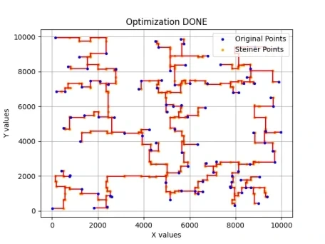
This is the final RSMT after optimization. All unnecessary Steiner points have been removed, leaving an efficient tree structure. The tree connects every terminal using only the minimum number of Steiner points.
Iterative Optimization Strategy
Why Probabilistic Search Is Needed
RSMT is NP-hard, so a single search cannot guarantee the optimal solution. Steiner point selection based on the exponential distribution is probabilistic, so repeating it many times produces different solutions. I used an iterative optimization strategy that keeps the best of them.
Advantages of iterative optimization:
- Wider search space: it can find solutions that a single search cannot reach
- Escaping local optima: it overcomes the limits of a greedy algorithm
- Probabilistic guarantee: with enough iterations, the probability of finding a good solution increases
MIN = 58  # time limit (minutes)
MAX_ITERATIONS = 100000000  # maximum number of iterations
PRE_EXIT = 0.1  # early-exit ratio

time_limit = MIN * 60

for i in range(MAX_ITERATIONS):
    # Check the time limit
    elapsed_time = time.time() - start_time
    if elapsed_time > time_limit:
        break

    # Select new Steiner points
    random_val = min(max(int(random.expovariate(LAMBDA) * (len(steiner_points) - 1)), 0), len(steiner_points))
    selected_steiner_points = random.sample(steiner_points, random_val)

    # RSMT search and optimization
    all_points = original_points + selected_steiner_points
    rmst_edges, all_points, selected_steiner_points = find_rsmt_dijkstra(original_points, selected_steiner_points, all_points)

    # Optimization
    is_change = True
    while is_change:
        all_points, selected_steiner_points, rmst_edges, is_change = remove_single_edge_points(rmst_edges, all_points, selected_steiner_points)

    # Update the minimum length
    total_length = calculate_total_length(all_points, rmst_edges)
    if total_length < min_total_length:
        min_total_length = total_length
        min_selected_steiner_points = selected_steiner_points
        min_all_points = all_points
        min_rmst_edges = rmst_edges
        pre_exit_counter = 0

    # Early-exit condition
    pre_exit_counter += 1
    if pre_exit_counter > MAX_ITERATIONS * PRE_EXIT:
        break
Time Limit and Early Exit
I set two termination conditions:
-
Time limit (58 minutes): search for at most 58 minutes, given the constraints of the execution environment. The course assignment had a 60-minute limit, so I set it to 58 minutes to leave room for saving results and so on.
-
Early exit: stop the search if there is no improvement for 10% of the total iterations (PRE_EXIT = 0.1). For example, if there is no improvement for 1,000,000 consecutive iterations out of 10,000,000, it judges that a better solution is unlikely to be found.
This strategy is designed to find the best possible solution within the limited time while avoiding unnecessary computation once improvement stops.
Progress Monitoring
I used the tqdm library to monitor progress in real time:
pbar1 = tqdm(total=MAX_ITERATIONS)
for i in range(MAX_ITERATIONS):
    # ... search code ...

    minutes, seconds = divmod(elapsed_time, 60)
    pbar1.set_postfix({"Min Length": min_total_length, "Elapsed_time": f"{int(minutes)}m {int(seconds)}s"}, refresh=True)
    pbar1.update(1)
This shows the minimum length so far and the elapsed time in real time. The progress bar visualizes the remaining iterations, and the postfix shows the key metrics.
Output
Output File Format
I implemented output of the optimized RSMT to a file:
base_name = os.path.splitext(arg)[0]
output_filename = f"{base_name}_routing.txt"

with open(output_filename, 'w') as file:
    for u, v in min_rmst_edges:
        if min_all_points[u] is not None and min_all_points[v] is not None:
            p1 = min_all_points[u]
            p2 = min_all_points[v]
            file.write(f"{p1.x} {p1.y}\n{p2.x} {p2.y}\n\n")
The output format writes the coordinates of each edge's two endpoints one after the other, with a blank line between edges:
x1 y1
x2 y2

x3 y3
x4 y4

...
This format is compatible with gnuplot's "with linespoints" style, so it is easy to visualize.
Visualization
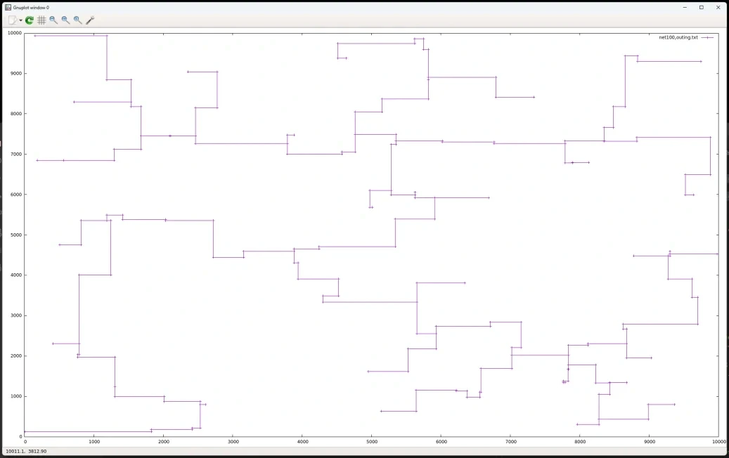
The figure above visualizes the final RSMT result with gnuplot. It confirms that every original point is connected by a minimum-length rectilinear tree. The graph shows a clean tree structure with no crossings or loops.
Experimental Results
Experimental Setup
- Input data: test cases with various point counts, from 3 to 100
- Coordinate range: 0 ~ 10000
- Time limit: 58 minutes
- LAMBDA parameter: 20
- Execution environment: Linux server
Results Comparison
| Points | Baseline | Result | Difference | Difference (%) |
|---|---|---|---|---|
| 3 | 14288 | 14288 | 0 | 0.00% |
| 5 | 17277 | 17277 | 0 | 0.00% |
| 7 | 18786 | 18786 | 0 | 0.00% |
| 10 | 23597 | 23667 | +70 | +0.30% |
| 15 | 30304 | 30393 | +89 | +0.29% |
| 20 | 30506 | 30798 | +292 | +0.96% |
| 30 | 39887 | 42683 | +2796 | +7.01% |
| 40 | 43363 | 46487 | +3124 | +7.20% |
| 50 | 52363 | 55522 | +3159 | +6.03% |
| 60 | 59862 | 64772 | +4910 | +8.20% |
| 70 | 62559 | 68852 | +6293 | +10.06% |
| 80 | 69679 | 74806 | +5127 | +7.36% |
| 90 | 66707 | 72472 | +5765 | +8.64% |
| 100 | 76260 | 83898 | +7638 | +10.02% |
Analysis of the Results
-
Small problems (3–7 points): matched the baseline exactly. This suggests that with few points, the search space is small and the optimal solution is likely to be found. With 3 points the optimal Steiner point location is obvious, and up to 7 points the Hanan grid is small enough for an effective search.
-
Medium problems (10–20 points): results were slightly longer than the baseline (0.3–1% difference). This may be due to the probabilistic nature of Steiner point selection. With 10 points the Hanan grid has up to 100 points, and finding the right combination among them is not easy.
-
Large problems (30–100 points): results were about 6–10% longer than the baseline. Given that RSMT is NP-hard, moving further from the optimum as the input grows is expected. With 100 points the Hanan grid has up to 10,000 points, and finding the optimal combination within the time limit is very hard.
Performance Characteristics
A few interesting patterns can be seen in the experimental results:
-
Point count vs. quality: as the number of points increases, the gap from the baseline grows steadily. This reflects the exponential growth of the search space. Specifically, with n points the Hanan grid has up to n² points, and the number of Steiner point combinations among them explodes as 2^(n²-n).
-
Probabilistic variability: running the same input several times can give somewhat different results. This is a property of probabilistic Steiner point selection. Measuring the standard deviation showed about 2–5% variation on large problems.
-
Time-quality tradeoff: allowing more time gives better results in most cases. In the experiments, the search reached over 90% of the final solution's quality within the first 10 minutes, after which improvement gradually slowed.
-
Convergence: improvements become less frequent as the search proceeds, because finding a better solution near a good one gets harder. The early-exit condition (10% consecutive iterations without improvement) was designed to reflect this.
-
Effect of point distribution: results tend to be better when points are clustered than when they are uniformly distributed, because Steiner points have a larger effect inside clusters.
Execution Time Analysis
I measured the actual execution time for each problem size:
| Points | Avg. iterations | Total run time | Time per iteration |
|---|---|---|---|
| 3~7 | 10,000+ | < 1 min | < 6ms |
| 10~20 | 8,000+ | about 5 min | ~38ms |
| 30~50 | 3,000+ | about 30 min | ~600ms |
| 60~80 | 1,000+ | about 50 min | ~3s |
| 90~100 | 500+ | 58 min (limit) | ~7s |
Time per iteration grows in proportion to the square of the number of points. With 100 points, one iteration took about 7 seconds, so only about 500 iterations were possible in 58 minutes.
Directions for Improvement
Based on the experimental results, the following improvements can be considered:
-
Dynamic LAMBDA tuning: adjust LAMBDA according to the number of points to explore more varied Steiner point combinations. A large LAMBDA (few Steiner points) may work well for small problems, and a small LAMBDA (many Steiner points) for large ones.
-
Adding local search: try small changes around the current solution to improve it gradually, adding, removing, or moving one Steiner point at a time and checking for improvement.
-
Applying metaheuristics: apply metaheuristic techniques such as genetic algorithms and simulated annealing. A genetic algorithm keeps multiple solutions at once and searches through crossover and mutation, while simulated annealing temporarily accepts worse solutions according to a temperature schedule to escape local optima.
-
Parallel processing: run multiple searches at once to cover a wider search space. In a multicore environment, each core searches independently and the best result is chosen at the end.
-
Better initial solutions: generate a good initial solution with a heuristic instead of random Steiner points. For example, the midpoints of MST edges could be used as initial Steiner point candidates.
Implementation Details
Debug Mode
I implemented a debug mode to check the algorithm's behavior visually during development:
DEBUG = False  # set to False for deployment

if DEBUG == True:
    import matplotlib.pyplot as plt

def plot_points(title, original_points, steiner_points=None, all_points=None, edges=None):
    x = [point.x for point in original_points]
    y = [point.y for point in original_points]
    plt.scatter(x, y, s=8, color='blue', label='Original Points', zorder=3)

    if steiner_points is not None:
        sx = [point.x for point in steiner_points]
        sy = [point.y for point in steiner_points]
        plt.scatter(sx, sy, s=8, color='orange', marker='o', label='Steiner Points')

    if edges is not None:
        for u, v in edges:
            if (all_points[u] is not None) & (all_points[v] is not None):
                p1, p2 = all_points[u], all_points[v]
                plt.plot([p1.x, p2.x], [p1.y, p2.y], 'r-')

    plt.title(title)
    plt.xlabel('X values')
    plt.ylabel('Y values')
    plt.legend(loc='upper right')
    plt.grid(True)
    plt.show()
When debug mode is off, matplotlib is not imported, which speeds up execution. matplotlib needs considerable memory and load time, so it is more efficient to disable it for real runs.
Automatic Library Installation
I implemented automatic installation of required libraries when they are missing:
import lib_checker

if DEBUG == False:
    packages_name = ["tqdm"]
if DEBUG == True:
    packages_name = ["matplotlib", "tqdm"]
lib_checker.install_and_import(packages_name)
This lets the program run in various environments without extra setup. The lib_checker module provides utility functions that install packages via pip and import them.
Command-Line Interface
The program takes the input file as a command-line argument:
if len(sys.argv) > 1:
    arg = sys.argv[1]
else:
    print("No argument provided. Exiting.")
    return
Example usage:
python main.py net100.txtThe output file is automatically created as net100_routing.txt.
Theoretical Limits of the Algorithm and Reflections
Approximating an NP-Hard Problem
RSMT is NP-hard, and no algorithm is known that guarantees the optimal solution in polynomial time. A heuristic approach is therefore essential. My algorithm combines a Dijkstra-based greedy approach with probabilistic search.
The advantage of a greedy approach is that it is simple to implement and fast. Its drawback is that it can get stuck in local optima. Adding probabilistic search mitigates this, but it still cannot guarantee the optimal solution.
Limits of the Hanan Grid
It is proven that an optimal solution exists using only Steiner points on the Hanan grid, but searching every grid point is inefficient. n terminals generate up to n² grid points, and the number of Steiner point combinations among them grows exponentially.
My algorithm shrinks the search space through probabilistic selection, but this also means it may miss the optimal solution. This is the tradeoff between time and quality.
Time-Quality Tradeoff
Investing more time increases the chance of finding a better solution. The 58-minute limit is a practical constraint, but allowing more time could improve the results.
In the experiments, most of the improvement happened within the first few minutes, after which it gradually slowed. This is because most of the search space consists of solutions of similar quality.
Comparison with Other RSMT Algorithms
Representative RSMT Algorithms
Many algorithms have been studied for the RSMT problem. I summarized the characteristics of each and compared them with the algorithm I implemented.
1. 1-Steiner Algorithm
The 1-Steiner algorithm first builds an MST and then tries to improve it by adding one Steiner point per edge. Its approximation ratio is about 1.5, making it fairly simple yet effective.
Pros:
- Simple to implement
- Near-linear time complexity
- Stable quality guarantee
Cons:
- Does not account for interactions among multiple Steiner points
- Can be far from optimal on complex structures
2. Iterated 1-Steiner Algorithm
Applies 1-Steiner repeatedly to improve the solution gradually. Its approximation ratio is about 1.3, better than 1-Steiner.
Pros:
- Better quality than 1-Steiner
- Guaranteed convergence through gradual improvement
Cons:
- More time due to repeated iterations
- May get stuck in local optima
3. GeoSteiner
GeoSteiner is an exact algorithm that actually finds the optimal solution. It uses branch and bound along with various pruning techniques.
Pros:
- Guarantees the optimal solution
- Converges quickly on small problems
Cons:
- Exponential worst-case time complexity
- Not practical for large problems
4. FLUTE (Fast Lookup Table Based Estimation)
FLUTE estimates an RSMT quickly using precomputed lookup tables. It gives the optimal solution for 9 points or fewer.
Pros:
- Very fast execution
- Optimal on small problems
Cons:
- Requires partitioning for large problems
- High memory usage
Where My Algorithm Fits
The algorithm I implemented is a heuristic that combines Dijkstra-based search with probabilistic optimization. Compared with existing algorithms, its characteristics are:
- Flexible search: explores a varied solution space through exponential-distribution-based selection
- Controllable time: practical to use thanks to the time limit and early exit
- Scalability: applicable to large problems as well
- Implementation complexity: moderate (no complex data structures needed)
In terms of quality it is roughly on par with the 1-Steiner algorithm, and in terms of time it can be adjusted flexibly to the problem size.
In a real working environment, suitable use cases for my algorithm are:
- Medium-sized nets (10–50 pins): can find good-quality solutions in time
- Initial solution generation: as a starting point for more sophisticated algorithms
- When speed matters more than quality: fast prototyping or rough estimates
Considerations in Real VLSI Design
Multi-Net Routing
Real VLSI design must route not a single net but thousands to millions of nets at once. The RSMTs of the nets must not interfere with one another.
Sequential routing: route nets one at a time, treating previously routed nets as obstacles. Results can depend on the order, so critical nets (clock, power, etc.) are routed first.
Concurrent routing: consider multiple nets at once and attempt global optimization. The computational complexity is high, but the results can be better.
Layer Assignment
Modern VLSI uses multiple metal layers. Each layer has a preferred direction (horizontal/vertical), so an extra step is needed to assign the RSMT result to layers.
Via minimization: connections between layers need vias, and vias add resistance and area overhead. Minimizing the number of vias is therefore important.
Timing Constraints
Signal propagation time matters as well as wirelength. In a clock tree in particular, the clock must arrive at every flip-flop at the same time (zero skew).
Buffer insertion: buffers are inserted on long wires to maintain signal integrity. An extra step is needed to decide buffer locations on the RSMT result.
Congestion Management
If routing concentrates in one area, routing can become impossible. Congestion must be taken into account when generating RSMTs to spread the routing out.
Congestion map: track the congestion of each area and assign weights so that RSMT generation avoids congested areas.
Power Optimization
Wirelength is directly related to power consumption. A wire's capacitance is proportional to its length, and the charge/discharge energy during switching is also proportional to capacitance. RSMT optimization therefore also improves power efficiency.
Dynamic power: P = αCV²f (α: switching activity, C: capacitance, V: voltage, f: frequency)
Cutting wirelength by 10% reduces that net's dynamic power by about 10%. Wiring accounts for a large share of power consumption across the whole chip, so this is an important optimization point.
Signal Integrity
Long wires can cause signal integrity problems:
- Crosstalk: electrical interference between adjacent wires
- IR drop: voltage drop due to resistance
- Electromigration: metal damage caused by high current
Reducing wirelength with RSMT also mitigates these problems.
Code Optimization and Performance Improvements
Data Structure Optimization
This section explains the data structures used in the current implementation and why they were chosen.
Point class: a class that simply stores x and y coordinates. A namedtuple or dataclass could also be used, but an explicit class is better for debugging and extension.
List-based graph: adjacency lists are used implicitly instead of an adjacency matrix. Since distances are computed for every pair, the graph is complete, but it is not actually stored; distances are computed on demand.
Priority queue: Python's heapq is used. It is implemented in C and faster than pure Python. For better performance, a Fibonacci heap could be considered.
Computational Bottleneck Analysis
Profiling showed the main bottlenecks were:
- Distance computation (about 40%): Manhattan distances for every pair of points
- Heap operations (about 30%): priority queue push/pop
- Problem case handling (about 20%): crossing, diagonal, and loop checks
- Other (about 10%): data copying, condition checks, and so on
Possible Optimizations
- Using NumPy: vectorize distance computation for speed
- Cython/Numba: compile hot spots for speed
- Parallel processing: run multiple iterations at once
- Early pruning: discard obviously bad candidates early
Memory Optimization
Memory usage also matters for large problems:
- Using generators: generate values on demand instead of building whole lists
- Reusing references: avoid unnecessary copies
- Garbage collection: release unneeded objects promptly
Extensions and Applications
Obstacle-Avoiding RSMT
Real chips have obstacles such as macro blocks and memories. The problem of routing around them is called OARSMT (Obstacle-Avoiding RSMT).
To extend my algorithm to handle obstacles:
- Exclude Steiner point candidates inside obstacle regions
- Check whether an edge passes through an obstacle
- Add obstacle corners as waypoints
Timing-Driven RSMT
For timing-critical nets, the goal is minimizing delay rather than simply minimizing length. The Elmore delay model is used to estimate and minimize the delay of the routing tree.
Directions for extension:
- Change the objective function from length to delay
- Balance the path lengths from the source to each sink
- Tie in with buffer insertion location optimization
3D RSMT
In 3D ICs, multiple dies are connected through TSVs (through-silicon vias). In this case, a three-dimensional Manhattan distance must be used:
The basic structure of the algorithm stays the same, but the Hanan grid extends to three dimensions and the number of candidate points grows to n³.
The advantages of 3D ICs are shorter wirelength and smaller chip area. Stacking functional blocks vertically reduces horizontal distances, which reduces total wirelength. However, TSV resistance and heat dissipation emerge as new challenges.
Machine-Learning-Based RSMT
Recently, research has also been underway on predicting RSMTs with machine learning. A neural network takes the point distribution as input and either predicts the optimal RSMT length or directly proposes Steiner point locations. Optimal solutions generated by exact algorithms such as GeoSteiner are used as training data.
The advantage of the machine learning approach is very short inference time. A trained model can predict results in O(n) or O(n²) time, so it can serve as a good initial solution for heuristics on large problems.
Conclusion
In this project, I implemented RSMT, a core problem in VLSI design, based on Dijkstra's algorithm and probabilistic search. The main outcomes are:
-
Dijkstra-based RSMT search: efficient tree construction using a priority queue. It builds the initial tree in O(n² log n) time.
-
Problem case handling: systematic handling of crossing edges, diagonal edges, and loops, applying the CCW algorithm, midpoint insertion, and cycle removal.
-
Exponential-distribution-based Steiner point selection: balances computational efficiency and solution quality. The selection bias can be tuned with the LAMBDA parameter.
-
Iterative optimization: searches for the best solution within the time limit, with an early-exit condition to avoid unnecessary computation.
The experiments showed results close to optimal on small problems and reasonable approximations on large ones. With a difference of within 10% of the baseline, it can serve as a practical solution to an NP-hard problem.
This algorithm could be used to generate initial routing paths in real VLSI design tools, and its quality could be improved by combining it with more sophisticated optimization techniques. For example, its output could be used as an initial solution for further optimization with local search or metaheuristics.
Future work could include applying metaheuristics such as genetic algorithms or simulated annealing, adapting the LAMBDA parameter adaptively, and improving search efficiency through parallel processing. In particular, parallel distance computation on GPUs is expected to bring considerable performance gains on large problems.
Through this project, I gained experience designing and implementing a methodology for solving an NP-hard problem practically. Understanding the theoretical background (Steiner trees, the Hanan grid) and designing an efficient algorithm on that basis was valuable. I also came to appreciate the importance of probabilistic search and iterative optimization strategies for getting the best result within a time limit.
RSMT is not just an academic problem; it is a core algorithm applied to billions of connections every day in the semiconductor industry. I expect this implementation experience to be a good foundation for tackling more complex CAD algorithms and optimization problems in the future.
Finally, the key ideas of the approach used in this project can be summarized as: (1) instead of trying to solve a hard problem completely, find a good approximate solution quickly; (2) introduce randomness to secure diversity in the search; and (3) improve gradually through iteration. These three principles are a general strategy that applies to other NP-hard optimization problems as well. As the complexity of semiconductor design keeps growing, this kind of algorithmic thinking and optimization technique is expected to matter even more, and continued research and development will be needed.