1. Design Topic
Designing a position controller for a DC motor
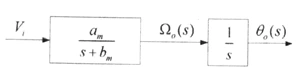
Figure 1. Servo motor transfer function model
Figure 1 above is the transfer function model of the servo motor used in the design. Here am is 600 and bm is 30. Ω0 is the motor speed, and an integrator is attached to that speed so that the system finally outputs the motor position θ0. A controller is added to this system to control it.
2. Design Constraints
-
Economic constraint: keep the capacity of the amplifier driving the motor as small as possible to keep cost low. (Keep K as small as possible.)
-
Productivity and durability: the system must reach the target (step input) as quickly as possible. The controller must also let the motor be used for as long as possible. (Keep oscillation as low as possible, i.e., a short settling time.)
-
The damping ratio of the closed-loop dominant poles must be between 0.4 and 0.7, and the settling time must be less than 1/30 sec.
-
The phase margin should be as large as possible (at least 40 degrees).
-
If the economic constraint conflicts with productivity and durability, assume a cost for each (and explain the assumptions) and minimize the total cost.
3. Design Process
1) Choosing the Controller
The transfer function of the given plant can be written as follows.
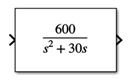
Figure 2. Servo motor transfer function
The denominator is second order, and adding a PI or PID integrator would push it to third order or higher. A design like that requires approximating a third-order-or-higher system as second order to find the parameters. So, for ease of design, I chose PD control. Using a PD controller also improves the stability of the system and gives good dynamic response (faster transient response and less overshoot).
Below is the system model including the PD controller.
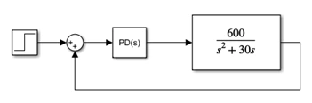
Figure 3. System model
2) Setting the Parameters
Damping factor
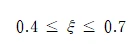
ωn
ωn can be found from the given settling time.
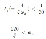
Rearranged, ωn can be written as an expression in ξ. In other words, once ξ is chosen, ωn is determined as well.
P.O.
P.O. can be expressed in terms of ξ, and substituting ξ gives the following range.
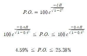
Kp, Kd
Kp and Kd can be found by rearranging the second-order system equation. Rearranging the system in Figure 3 above gives the following.
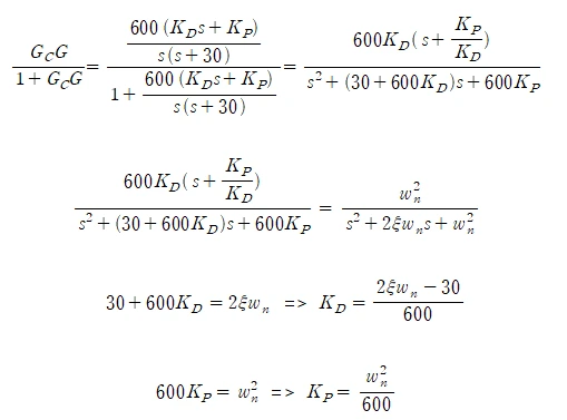
Kd can be expressed in terms of ξ and ωn, and Kp in terms of ωn.
This shows that all of the parameters above are determined once ξ is chosen. Figure 4 below shows the range of each parameter as ξ varies, computed in Excel.
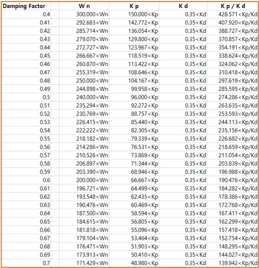
Figure 4. Parameter ranges
Here Kp/Kd is obtained by dividing the Kp range by the Kd range.
3) Finding the Gain with the Root Locus
A root locus is a graph of how the pole locations of a system move as one of its parameters changes. Here the parameter is the gain K. A second-order system has two gains, Kd and Kp, so one value has to be fixed.
By picking ξ and Kp/Kd and finding the point on the root locus that satisfies them, the Kd gain of the system can be found. Why the root locus is used to find Kd rather than Kp can be seen from the rearranged equation in Figure 5.
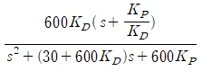
Figure 5. Closed-loop transfer function of the system
To use the root locus, the gain being solved for is pulled out in front. Figure 5 shows that Kd can be factored out of the fraction, so I find the Kd gain first. Of course, once Kp/Kd and Kd are determined, Kp follows automatically.
First, with a damping factor of 0.55, I set Kp/Kd to 230, which is greater than 226.682 from the range in Figure 4, and ran the simulation. The result is shown in Figure 6.
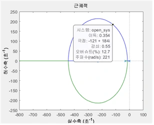
Figure 6. Root locus for damping factor = 0.55, Kp/Kd = 230
Finding the point on the root locus where the damping factor equals the chosen 0.55 gives the gain. The gain at that point is 0.354, and this is the Kd gain. The P.O. at this point satisfies the following.

4) Checking the Requirements
With the Kd found in 3), I obtained the Bode plot and the output for a step input.
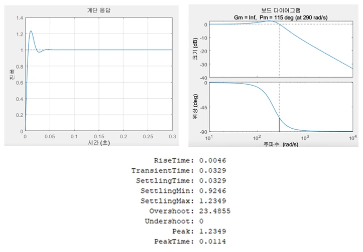
Figure 7. Bode plot and step response for damping factor = 0.55, Kp/Kd = 230
Figure 7 shows that the settling time just barely fits within the initially set 0.033333, and the phase margin satisfies the requirement at over 40 degrees.
The MATLAB code that produces the root locus, the Bode plot, and the step response is shown in Figure 8 below.
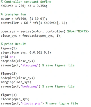
Figure 8. MATLAB code for damping factor = 0.55, Kp/Kd = 230
The variable KpDivKd means Kp/Kd and, like the damping factor, is set at the start.
Kd is the gain and is set to 1 when plotting the root locus. Once the gain is found from the root locus, that value is plugged in to get the step response and Bode plot.
motor is the transfer function of the plant, including the integrator, and controller is the transfer function of the PD controller.
open_sys is the transfer function of motor and controller connected in series, and it is the transfer function used for the root locus.
Connecting open_sys through the feedback function gave close_sys, the closed-loop transfer function.
figure(1), figure(2), and figure(3) were set up to output each plot separately.
Then step() gave the output for a step input, bodeplot() gave the Bode plot, and rlocus() gave the root locus plot.
stepinfo() was used to see parameters such as RiseTime and SettlingTime.
Beyond that, I used grid settings and the saveas() function to save the figures.
5) Finding the Optimal Values
Step 4) found a result that meets the requirements, but for an optimal design I simulated many values. Figure 9 below is a table summarizing the simulation results. It was produced by repeating steps 3)–4). The detailed figures, code, and process are included in section 6, Appendix.

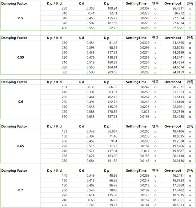
Figure 9. Changes in values with damping factor and Kp/Kd
First, I chose a damping factor of 0.7. The reason is shown in Figure 10 below. As ξ increases, the system's overshoot decreases, so I picked 0.7, which has the least overshoot and oscillation.
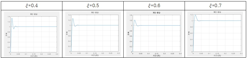
Figure 10. Overshoot versus damping factor
With a damping factor of 0.7, K and settling time are in conflict. In other words, the economic constraint is in conflict with productivity and durability. So I had to find a compromise between them.
Cost from K
K is a gain, so it has to be produced with an amplifier. Assume the LM741, one of the most widely used op-amps.

Figure 11. Gain of the LM741
This chip can provide a gain of at least 50 and at most 200. Think of using one for Kd and one for Kp. On Amazon the chip costs $12.52 (about ₩16,927) for 20. That is ₩846 each, and two are needed, so ₩1,692. To get high gain while minimizing cost, Kp and Kd have to stay below 200. If either goes above 200, another chip is needed for the extra gain.
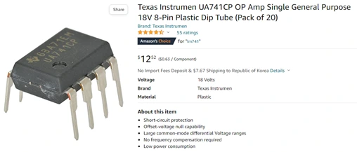
Figure 12. Price of the LM741
Cost from Productivity and Durability
A servo motor operated at a surface temperature of 80 degrees can be used for up to 50,000 hours.
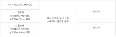
Figure 13. Servo motor lifetime
Using the motor below from Devicemart, a servo motor costs ₩6,500.

Figure 14. Servo motor price
Cost Estimate
Based on the results above, the cost comes out as follows.
The maximum operating time is assumed to be 20,000 hours.
Op-amp cost: ₩1,692
Motor cost: ₩6,500
Increasing K further would require more op-amps and raise the op-amp cost, so the optimum is to use one op-amp each for Kp and Kd. Each gain must also stay below 200. On this basis, I could select the following values.
6) Final Design Result
The parameters of the final design are shown in Figure 15 below.

Figure 15. Final parameters
The resulting Bode plot and step response are shown in Figure 16 below.
The settling time is 0.0144, less than 0.03, so it meets the requirement. The damping factor of 0.7 also meets the requirement, and the phase margin is 128 degrees, greater than 40 degrees. K is set to an appropriate value considering cost, productivity, and durability.
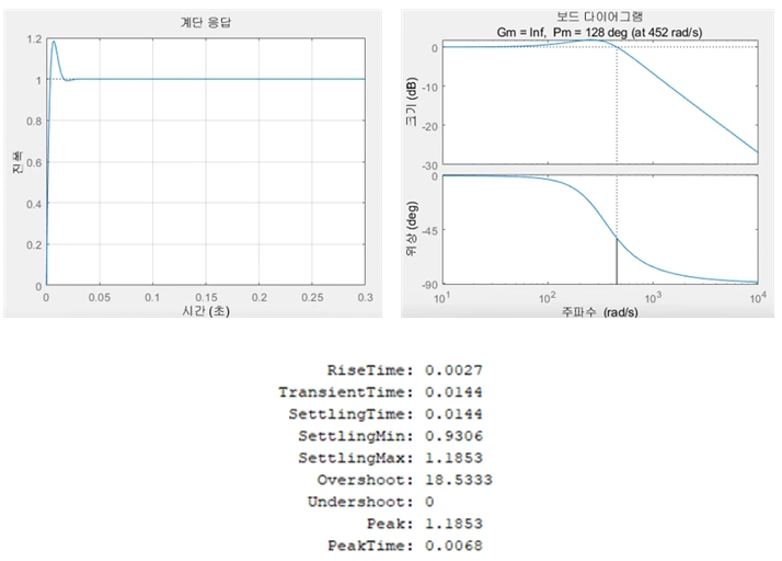
Figure 16. Bode plot and step response for damping factor = 0.7, Kp/Kd = 260
4. Reflections
I designed a position controller for a DC motor using a PD controller. I set each parameter and in the process used the root locus, the Bode plot, and the step response. The result met all of the given design constraints for settling time, damping factor, and phase margin. The economic constraint conflicted with productivity and durability, and I designed with cost in mind.
If I had chosen the values considering only K (cost) versus settling time (productivity and durability), the result would have been as follows.
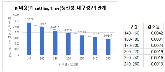
Figure 17. Kp/Kd versus settling time
The rate of decrease per interval in Figure 17 gets smaller and smaller. This means that as K grows, i.e., as cost increases, the performance gained per unit cost shrinks. So I thought the intervals 140–160 and 160–180, which show a large decrease relative to cost, were worth the investment. That is why I chose Kp/Kd = 180.
The parameters of this final design are shown in Figure 18 below.

Figure 18. Final parameters
The resulting Bode plot and step response are shown in Figure 19 below.
The settling time is 0.0216, less than 0.03, so it meets the requirement. The damping factor of 0.7 also meets the requirement, and the phase margin is 129 degrees, greater than 40 degrees. K is set to an appropriate value considering cost, productivity, and durability.
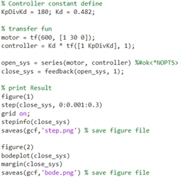
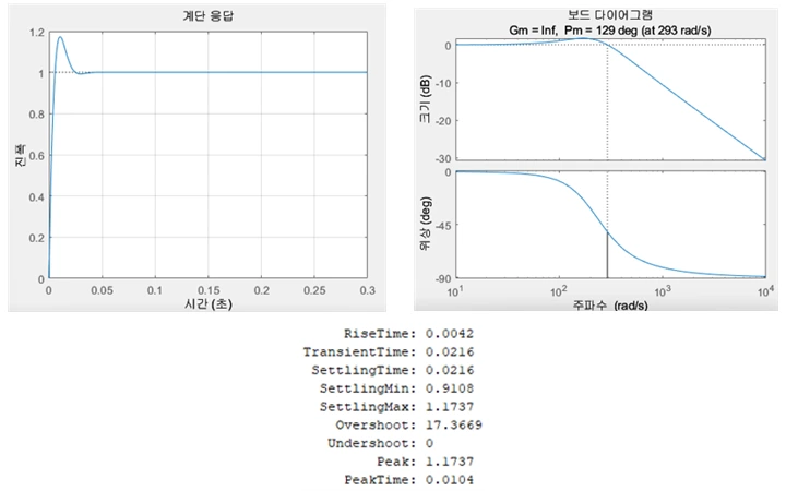
Figure 19. Bode plot and step response for damping factor = 0.7, Kp/Kd = 180
5. References
LM741 datasheet https://www.ti.com/lit/ds/symlink/lm741.pdf
What determines a motor's lifetime? (Korean) https://inaom.tistory.com/552
Texas Instrumen UA741CP OP Amp https://www.amazon.com/Texas-Instrumen-UA741CP-General-Purpose/dp/B01KO48D5K/ref=sr_1_3?keywords=ic+741&qid=1668714216&sr=8-3
Servo motor (Devicemart) https://www.devicemart.co.kr/goods/search?keyword_log_flag=Y&search_text=%EC%84%9C%EB%B3%B4%EB%AA%A8%ED%84%B0&q=%EC%84%9C%EB%B3%B4%EB%AA%A8%ED%84%B0&x=18&y=19
PID Controller, Proportional Integral Derivative Controller (Korean) http://www.ktword.co.kr/test/view/view.php?m_temp1=4670