1. Ways to Build a High-Performance Multiplier
Multiplication is generally more complex and slower than addition. Its speed can be improved in several ways. The approaches I considered were reducing the number of partial products with Booth Encoding and the TDM method.
According to "A method for speed optimized partial product reduction and generation of fast parallel multipliers using an algorithmic approach," TDM is a method that reduces partial products in three dimensions using vertical compressor slices.
V. G. Oklobdzija, D. Villeger, and S. S. Liu, "A method for speed optimized partial product reduction and generation of fast parallel multipliers using an algorithmic approach", IEEE Transactions on Computers, vol 45, no. 3. Institute of Electrical and Electronics Engineers (IEEE), pp 294–306, 3-1996.
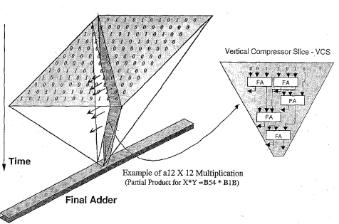
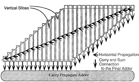
Figure 1 TDM multiplier
When I actually implemented the TDM multiplier, it did not perform as well as the Booth encoding approach. The reason is that I overlooked TDM's key idea: a carry is produced faster than a sum. With multi-input gates, the advantage of the carry being faster than the sum cannot be fully exploited. Below is the result of the multiplier designed with TDM.
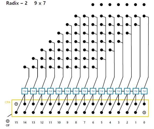
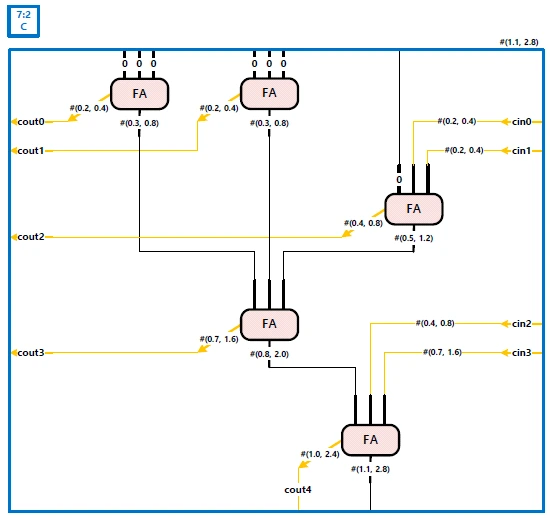

Figure 2 Partial products, the 7:2 compressor of the TDM multiplier, and the simulation result
This is the original TDM multiplier, which uses radix-2 and does not reduce the partial products at all. It is not faster than the Booth encoding approach, but combined with the Booth encoding described below, it further improved the multiplier's performance.
For Booth encoding, I considered radix-4, radix-8, and radix-16. I actually implemented radix-4 and radix-8, and during planning I confirmed that radix-16 would be slower than radix-4. For a 9x7 multiplication, the operands have few bits, so radix-4 is the most efficient.
1) radix-4
This is the multiplier I actually built. It is explained in detail in section 2.
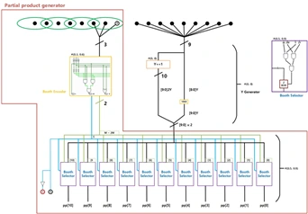
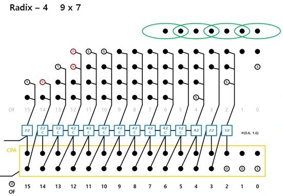
Figure 3 Booth encoding and partial products
2) radix-8
It has 4 partial product stages, the same as radix-4, so it is not faster. To handle 3Y, I came up with adding Y and 2Y 4 bits at a time.
For this method, I recommend checking out the other post. Read the post
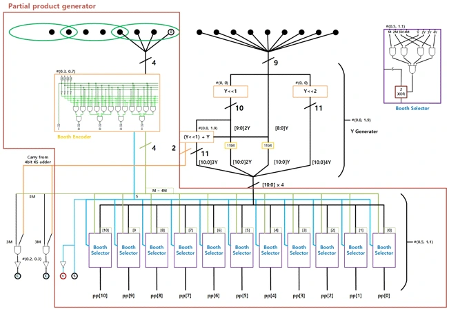
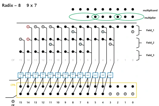
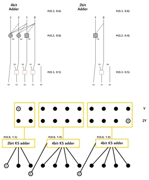
Figure 4 Booth encoding and partial products
3) radix-16
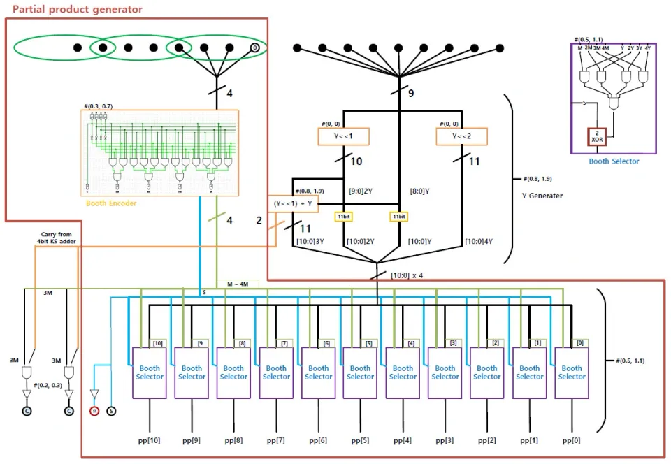
It can cut the partial product stages down to 2, but the Booth encoding stage takes a lot of time, so I found it is only worthwhile when the operands are large. All of ± Y ~ 7Y can be built by adding or subtracting a weight to or from a base. Generating the partial products takes #(1.9, 4.6).
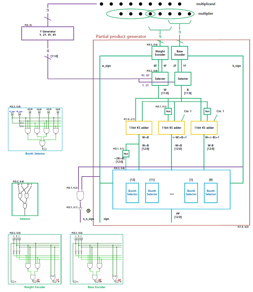
Figure 5 Booth encoding and partial products
In the end, I designed the radix-4 version. TDM reached a maximum of 3.6 ns, radix-4 a maximum of 3.4 ns, and radix-8 a maximum of 4 ns. Radix-16 is expected to take even longer.
2. The Multiplier I Designed
As explained above, I ended up designing the radix-4 version.
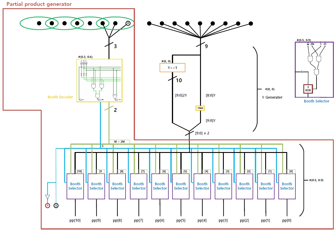
1) Booth Encoder
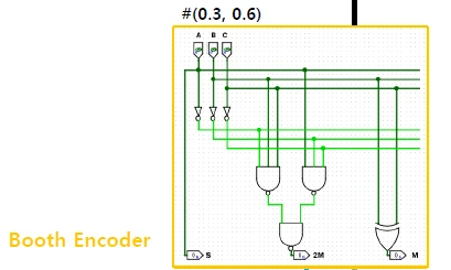
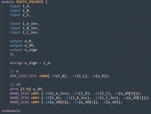
Figure 6 Booth encoder
The Booth encoder decides, for each group of 3 bits, whether the result is Y, 2Y, -Y, or -2Y. S is the sign bit. This result goes into the Booth selector below.
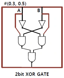
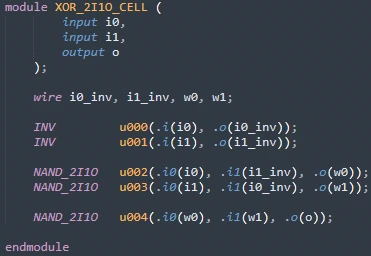
One XOR cell is used to produce M, which indicates Y. The XOR cell is implemented as shown in Figure 8.
Three 3-bit NANDs are used to produce 2M, which indicates 2Y.
* 2bit XOR Cell
2) Booth Selector
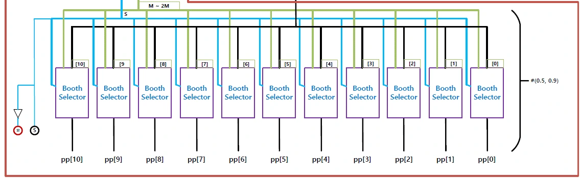
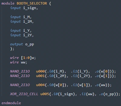
The Booth selector uses M and 2M from the Booth encoder to choose between Y and 2Y. It then takes the one's complement depending on the sign bit. To complete the two's complement, the sign bit is later added to the LSB of the partial product.
Three 2-bit NANDs are used to select Y or 2Y.
One XOR cell is used to take the one's complement.
3) Partial product generator
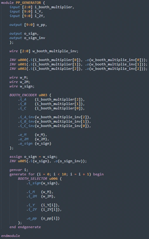
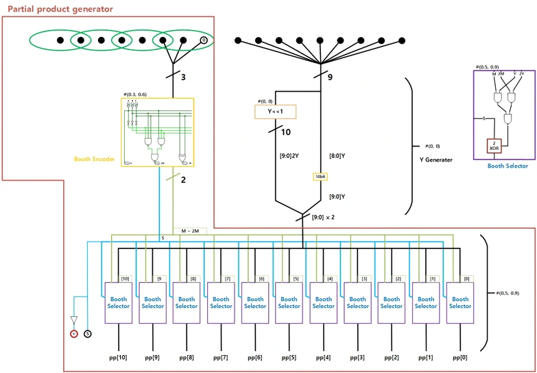
Figure 10 Partial product generator
The partial product generator instantiates the 1) Booth Encoder and 2) Booth Selector built above. The output of the Booth encoder feeds 10 Booth selectors, which produce and output the partial product.
4) Generating Y and 2Y
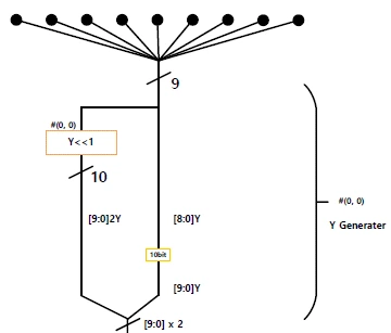

Figure 11 Generating Y and 2Y
Y and 2Y are declared as in Figure 11. 2Y requires a 1-bit left shift, which is implemented by appending a 0 at the LSB. This allows shifting without spending any extra gates.
5) Generating the Partial Products
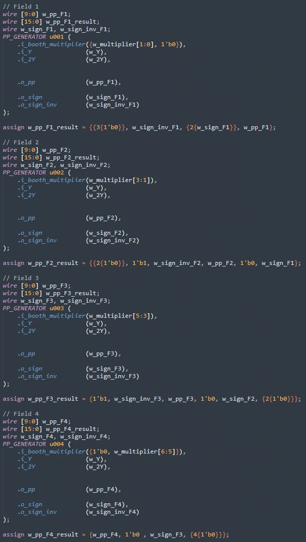
Figure 12 Generating the partial products
The partial products are generated by instantiating the 3) Partial product generator built above.
wire [9:0] w_pp_F1 ~ w_pp_F4 are the outputs of the partial product generator.
wire [15:0] w_pp_F1_result ~ w_pp_F4_result are those outputs aligned to their bit positions, including the sign bit, and extended to 16 bits.
6) Carry Save Adder
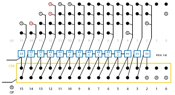
Figure 13 Partial products
The partial products from 1) ~ 5) above are reduced in number through carry save adding. For this, I designed a 4:2 compressor using the TDM technique.
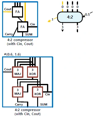
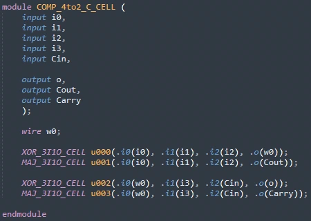
Figure 14 4:2 compressor (with Cin)
The 4:2 compressor in Figure 14 takes 4 partial product inputs and one Cin, and produces a Cout that goes into the next compressor, plus the Carry and Sum outputs. The Cout going to the next compressor finishes earlier than Carry and Sum, and feeding it into the next stage shortens the computation time. Figure 15 below shows the critical path of the 4:2 compressor.
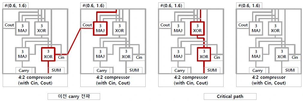
Figure 15 Carry propagation and the critical path
Figure 15 shows that passing through two XORs takes longer than propagating the previous carry. This is the advantage of a compressor cell built with TDM.
The other compressor cells used for carry save adding are as follows.
4:2 Compressor
A 4:2 compressor that does not take a carry in.
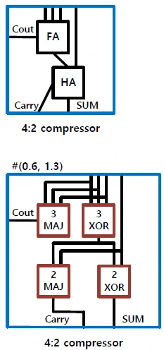
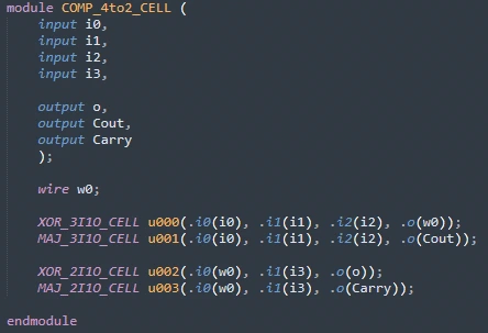
Figure 16 4:2 compressor
3:2 Compressor
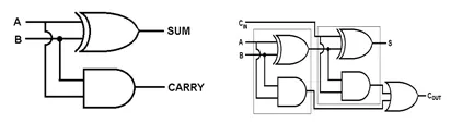
A 3:2 compressor with a carry in and one without. The 3:2 compressor, with or without a carry in, is the same as an FA.
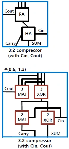
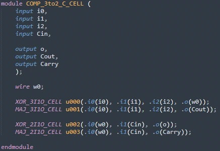
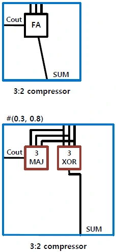
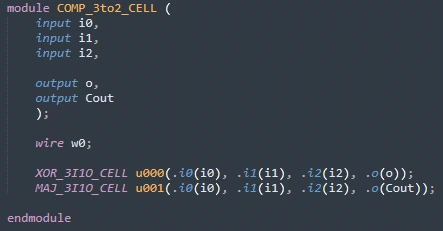
Figure 16 3:2 compressor (with Cin), 3:2 compressor
2:2 Compressor
The FA, a 2:2 compressor with a carry in, and the HA, a 2:2 compressor without one.
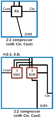
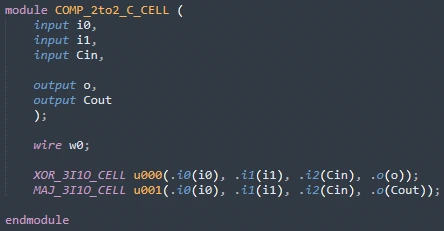
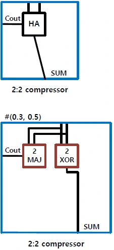
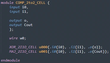
Figure 17 2:2 compressor (with Cin), 2:2 compressor
The XOR and MAJ cells used in the compressor cells are as follows.
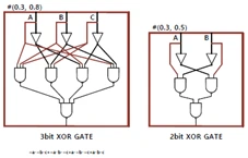
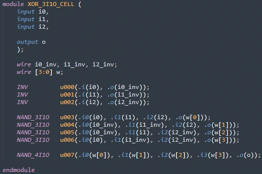
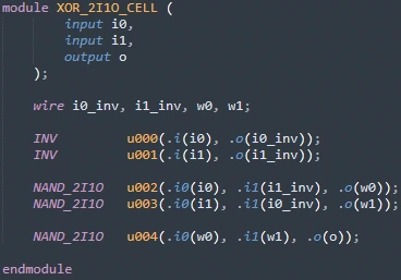
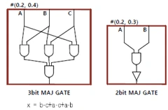
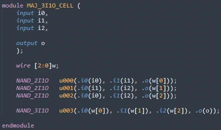
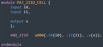
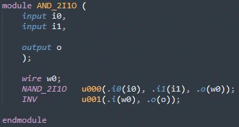
With these compressor cells, the partial products can be compressed as shown in Figure 20.
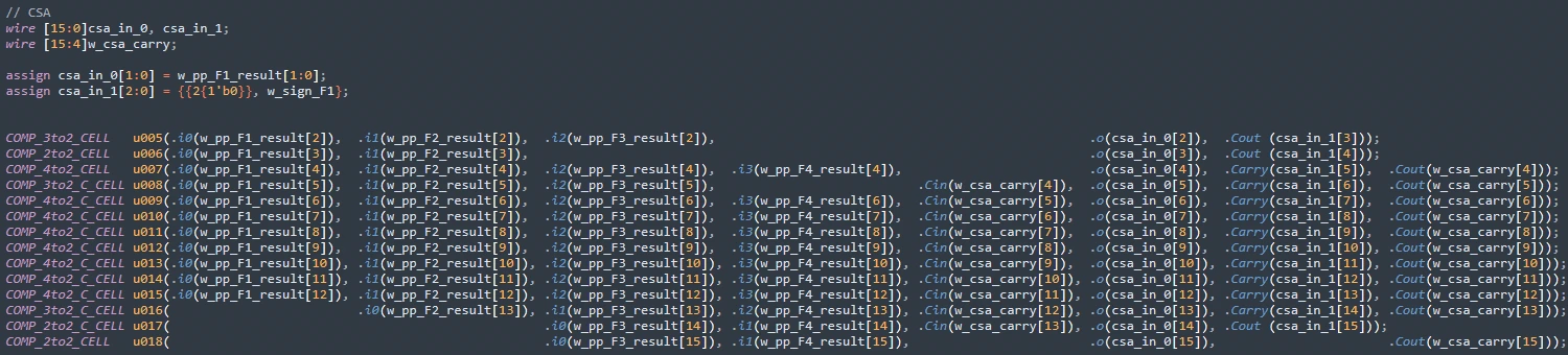
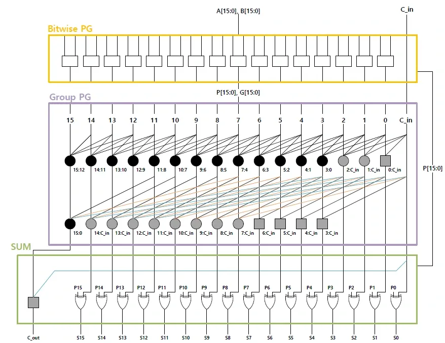
7) Carry Ripple Adder - Kogge-Stone Adder using Higher Valency Cell
Adding the compressed csa_in_0 and csa_in_1 with the Kogge-Stone Adder using Higher Valency Cell from my second design gives the desired result. That adder was explained in detail in the second report, so I skip the explanation here.
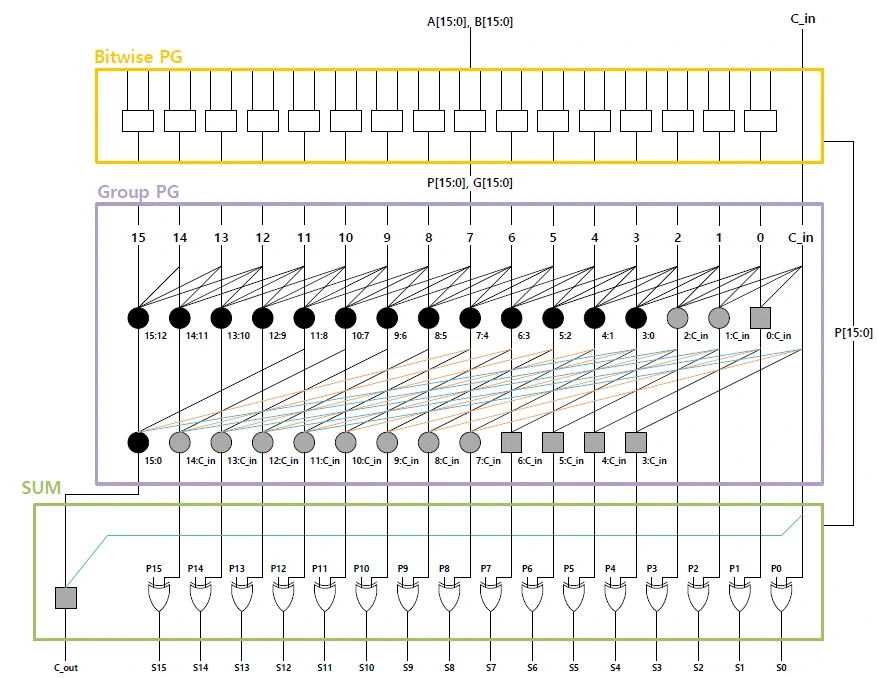
Figure 21 Kogge-Stone Adder using Higher Valency Cell
3. Result Waveforms / Accuracy Verification
1) How Accuracy Was Verified
I verified accuracy by writing a testbench that feeds every possible input into the multiplier.
[ Test Bench ]
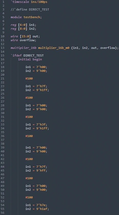
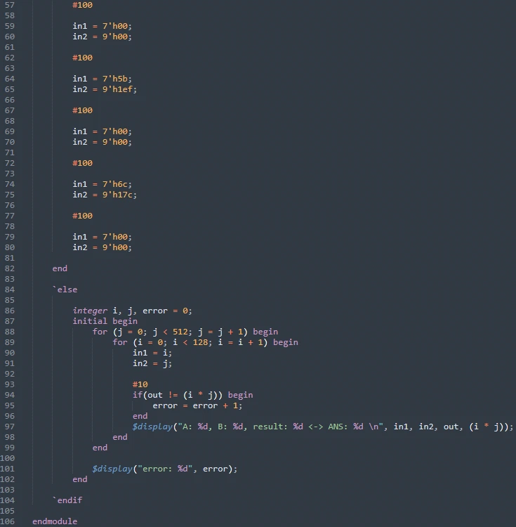
Figure 22 Testbench
The testbench is designed to run in two modes. By default, it runs code that tests every possible input to the multiplier. Uncommenting the `define statement at the very top switches to a simulation with manually entered values. These are the values given as design conditions. Below are the results with the `define statement commented out.
(1) Waveform at an arbitrary point

Figure 23 Result waveform in decimal
The waveform shows that the designed multiplier works without problems.
(2) Console output
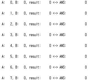
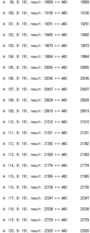
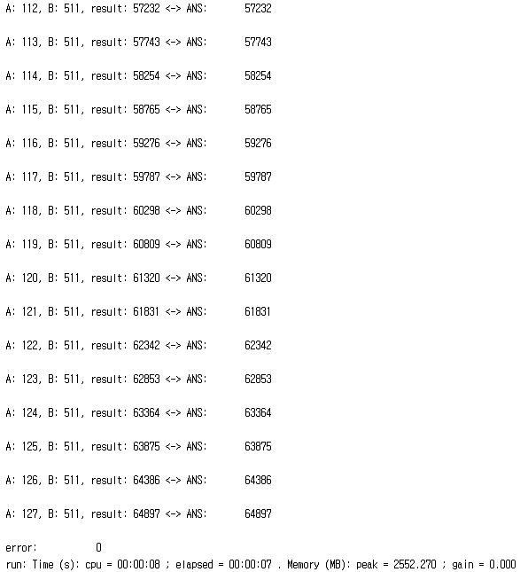
Figure 24 Console output
Figure 24 shows part of the console output. Everything is printed correctly, and error is 0, meaning the designed multiplier's results all match the expected answers.
2) Delay Analysis of the Designed Multiplier
Uncommenting the `define statement in the Figure 22 testbench and running it simulates the given values.

Figure 25 Result waveform in decimal
The results in Figure 25 show that the values are computed correctly.

Figure 26 Longest delay
The longest delay of the designed multiplier occurs when computing in1 = 7'h00, in2 = 9'h00 right after computing in1 = 7'h00, in2 = 9'h00, and it is 3.5ns.
Figure 27 below shows all the delays of the designed multiplier.
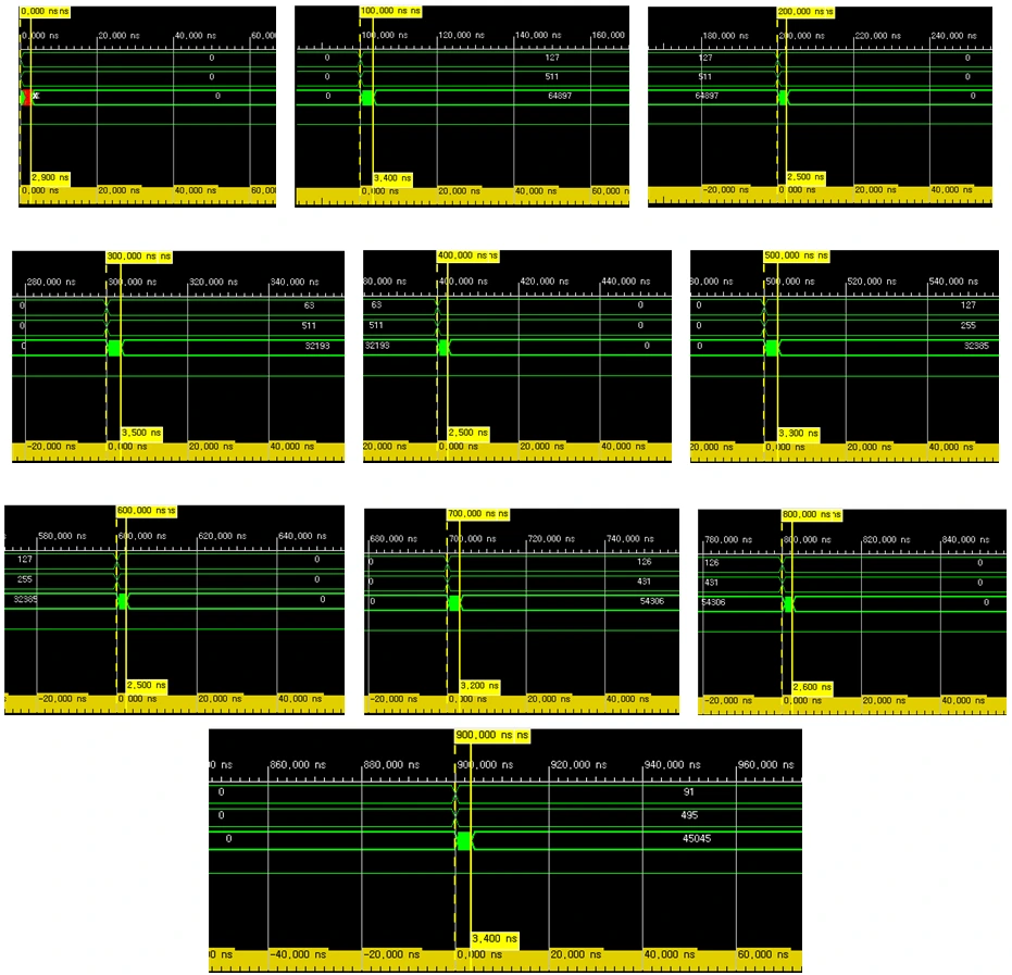
Figure 27 Delays
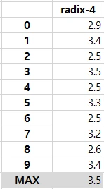
Figure 28 Delay summary table
3) Critical Path Analysis of the Designed Multiplier
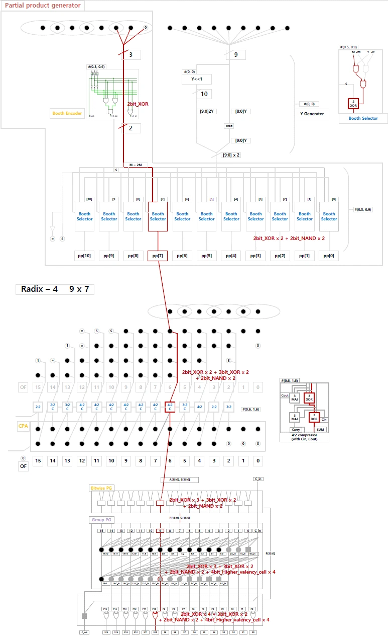
Figure 29 Critical path analysis
Figure 29 above shows the critical path of the designed multiplier. The Booth encoder uses two 2-bit XORs, and then the Booth selector uses two 2-bit NANDs. The resulting partial product passes through two 3-bit XORs in the 4:2 compressor. Finally, the CPA consumes one 2-bit XOR, four 4-bit higher valency cells, and one 2-bit XOR, in that order.
In other words, the path goes through at most four 2-bit XORs + two 3-bit XORs + two 2-bit NANDs + four 4-bit higher valency cells.
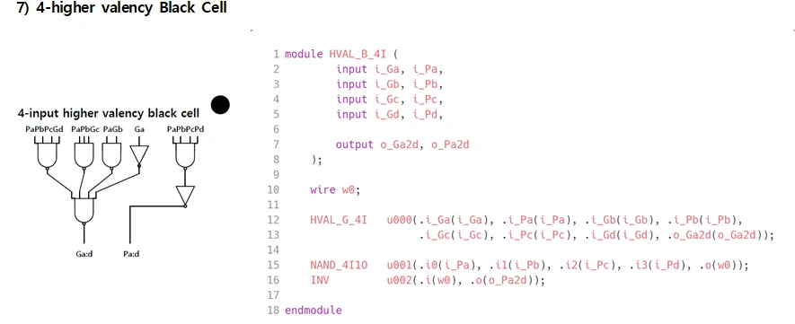
A 4-bit higher valency cell has a delay equal to two 4-bit NANDs.
4. Conclusion
I implemented Booth encoding with radix-4 and compressed the resulting partial products with TDM 4:2 compressors. Finally, I obtained the result with a Kogge-Stone Adder using Higher Valency Cell as the CPA.
Along the way, I designed the Booth encoder, Booth selector, CSA, CPA, and more.
The longest delay of the designed multiplier is 3.5ns.
The critical path that produces the longest delay goes through four 2-bit XORs + two 3-bit XORs + two 2-bit NANDs + four 4-bit higher valency cells.
I verified accuracy by writing a testbench that feeds every possible input into the multiplier. All results came out correct.
Through this design, I learned about various ways to build a high-performance multiplier, and building one myself taught me the principles in more detail. One regret is that I tried to design multipliers with radix-8 and radix-16, but because the operands have few bits, performance actually got worse, so I could not use them.