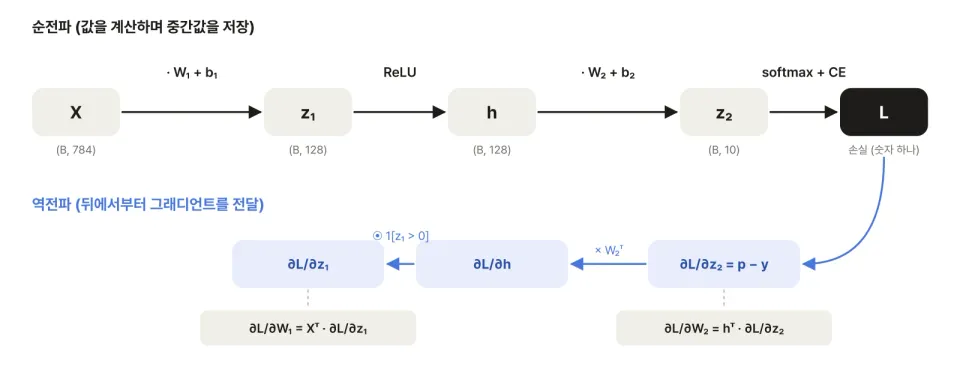
Neural Network Basics: From the Perceptron to Multilayer Networks

The 3 key points of this post

A neuron, the unit of a neural network, is a very simple computation: "multiply the inputs by weights and add them up (weighted sum), then pass that value through an activation function."
A single neuron (perceptron) can only solve problems that can be split by one straight line. When actually run, AND and OR reach 100% within a few epochs, but XOR keeps failing for all 20 epochs. Stack one more layer and XOR is solved too.
Learning means defining "how wrong we are (loss)" as a number and nudging the weights little by little in the direction that makes that number smaller (gradient descent). If the size of each step (learning rate) is too large, training diverges.

This is the first post in the AI Note series, which runs from CNNs to LLMs. Every model that comes later stands on the four things covered here: neurons, layers, loss, and gradient descent. The math is written so that high-school math (linear expressions, what a derivative means) is enough to follow along, and every example is a result I computed by hand or ran in code. The next post (Part 2) covers what is deferred here, "how to compute the gradient," that is, backpropagation.

1. Machine learning fits a function with data instead of rules

Suppose we want to build a program that looks at a photo of a handwritten digit and tells which of 0–9 it is. The traditional approach is for a person to write rules, such as "if the top is round and a straight line comes down, it's a 9." But everyone's handwriting is different, so the rules grow endlessly and exceptions keep appearing.

Machine learning flips the direction. Instead of writing rules directly, we prepare a function with lots of adjustable numbers (weights), show it labeled examples (data), and tune those numbers.

\text{image} \;\xrightarrow{\;f(\,\cdot\,;\,\text{weights})\;}\; \text{digit}

A neural network is one way to build this "adjustable function." Its smallest unit is the neuron.

2. A single neuron: weighted sum and activation

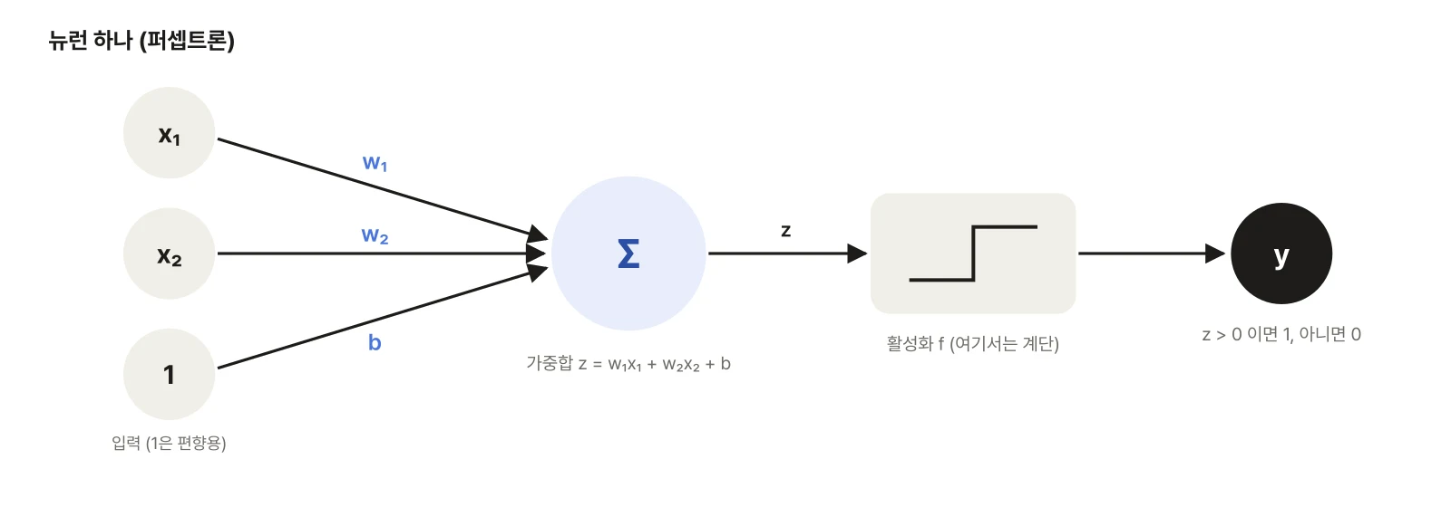
Structure of a single neuron. Inputs x1, x2 and the constant 1 are multiplied by weights w1, w2, b respectively and summed into the weighted sum z, which passes through a step function that outputs 1 if z is greater than 0 and 0 otherwise

A single neuron does its work in two steps.

Weighted sum: multiply each input by its weight, add them all up, and add the bias $b$ .

z = w_1 x_1 + w_2 x_2 + b

Activation: feed $z$ into the activation function $f$ to decide the output. The oldest form, the perceptron (Rosenblatt, 1958), uses a step function: 1 if $z > 0$ , otherwise 0.

y = f(z) = \begin{cases} 1 & (z > 0) \\ 0 & (\text{otherwise}) \end{cases}

You can think of the weight $w$ as "how important this input is," and the bias $b$ as "how easily the neuron outputs 1 (the threshold)."

Computing by hand: building AND

With $x_1, x_2$ each 0 or 1, let's build AND, which outputs 1 only when both are 1, using a single neuron. Setting $w_1 = w_2 = 1$ and $b = -1.5$ does it.

$x_1$	$x_2$	$z = x_1 + x_2 - 1.5$	$y$	AND
0	0	−1.5	0	0
0	1	−0.5	0	0
1	0	−0.5	0	0
1	1	0.5	1	1

Change the bias to $-0.5$ and $z > 0$ holds when even one input is 1, so it becomes OR. The key point is that the same neuron produces different logic just by changing its weights.

3. The perceptron splits with a single straight line

$z = w_1 x_1 + w_2 x_2 + b = 0$ is a straight line in the plane. The neuron effectively labels one side of this line 1 and the other side 0. So what happens with a problem that cannot be split by a single line?

Let's have the weights learned from data instead of set by hand. The perceptron learning rule is simple. Look at the samples one at a time, and only when the prediction is wrong, push the weights toward the correct answer ( $\eta$ is the size of each push).

w \leftarrow w + \eta\,(\text{target} - \text{prediction})\,x, \qquad b \leftarrow b + \eta\,(\text{target} - \text{prediction})

Starting from small random values with $\eta = 0.5$ , I trained it separately on AND, OR, and XOR (1 only when the two inputs differ).

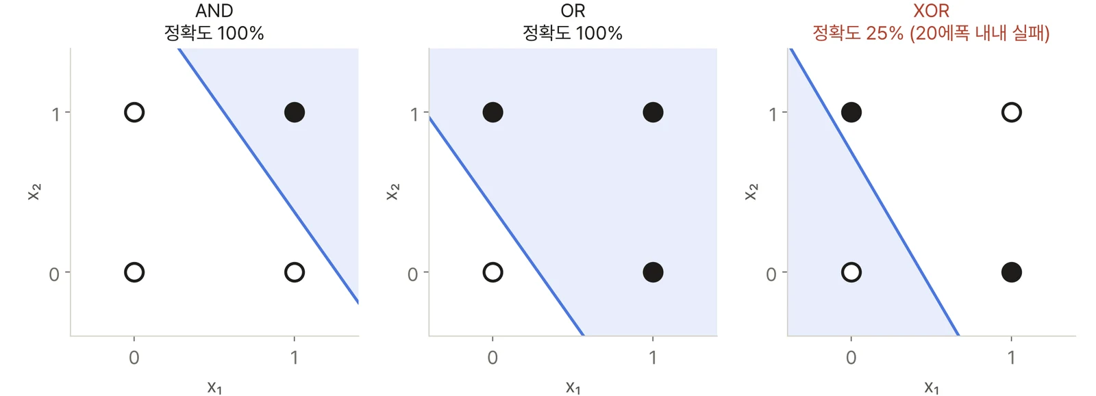
Decision boundaries learned by the perceptron. For AND and OR, a single line exactly separates the black dots (1) from the white dots (0) for 100% accuracy, while for XOR no line can separate the two diagonally placed pairs, so it fails for all 20 epochs

Problem	Result	Epochs taken	Learned weights $(w_1, w_2, b)$
AND	100% accuracy	8	(1.02, 0.72, −1.29)
OR	100% accuracy	6	(1.02, 0.72, −0.29)
XOR	Still failing after 20 epochs	−	The number of errors per epoch goes 3, 1, 3, 1, 3, 3, 4, 4, … and never reaches 0

For AND and OR, as in the figure, a single line separates the black dots (1) from the white dots (0). For XOR, the points labeled 1, $(0,1), (1,0)$ , and the points labeled 0, $(0,0), (1,1)$ , are crossed diagonally, so no line you draw can separate them. The perceptron learning rule is guaranteed to find a solution if the data is separable (the convergence theorem), but if it is not separable, it oscillates forever. After Minsky and Papert pointed out this limitation in 1969, neural network research went through a period of stagnation.

4. Stacking layers solves XOR

The solution is to stack neurons into layers. Put into words, XOR is "at least one of the two is 1 (OR), but not both are 1 (AND)." In Section 2, OR and AND could each be built with a single neuron. So place an OR neuron and an AND neuron in the first layer, and compute "OR and not AND" in the second layer.

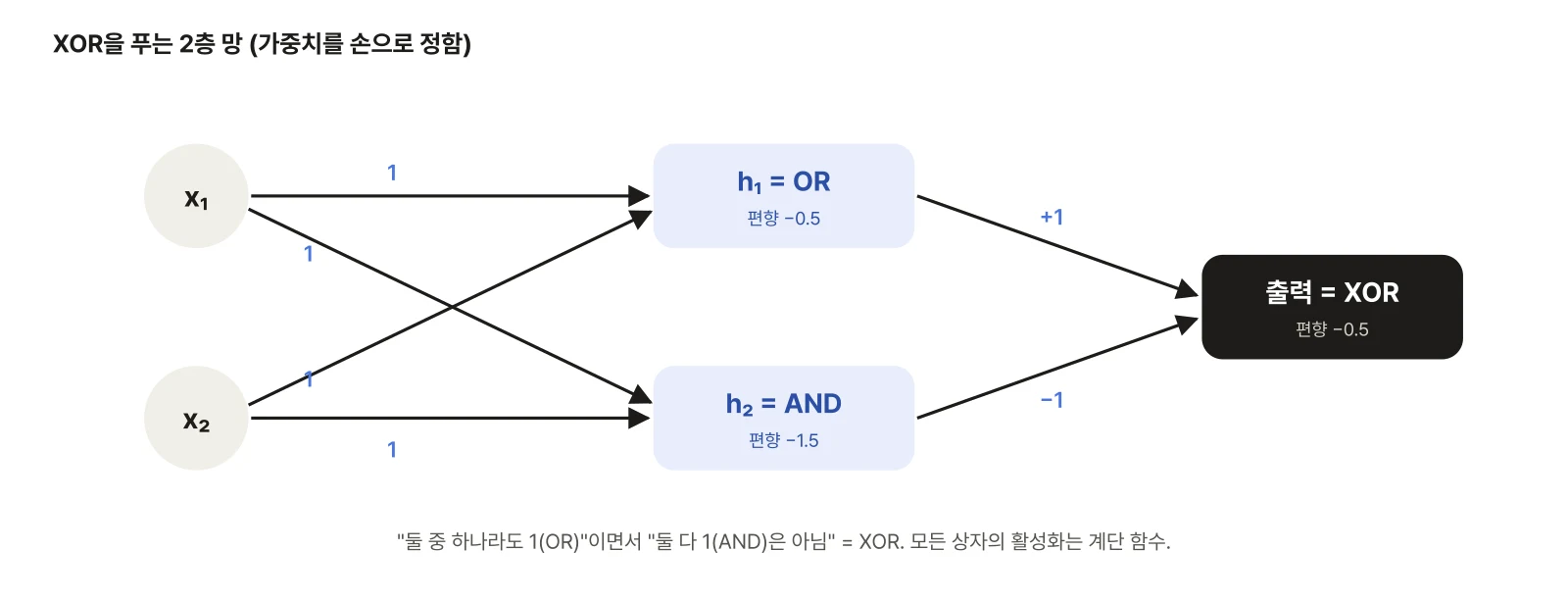
A two-layer network that solves XOR. Inputs x1, x2 go into an OR neuron (bias −0.5) and an AND neuron (bias −1.5), and the output neuron gives a weight of +1 to OR and −1 to AND and adds a bias of −0.5 to produce XOR

Trace all four inputs by hand and you really do get XOR. The output neuron is $z = h_1 - h_2 - 0.5$ .

$x_1$	$x_2$	$h_1$ (OR)	$h_2$ (AND)	$z = h_1 - h_2 - 0.5$	Output	XOR
0	0	0	0	−0.5	0	0
0	1	1	0	0.5	1	1
1	0	1	0	0.5	1	1
1	1	1	1	−0.5	0	0

Once the first layer turns the input into a new representation $(h_1, h_2)$ , the problem becomes an easy one for the second layer, separable by a single line. This is the core idea of the multilayer perceptron (MLP): with each layer, the problem is transformed into a representation that is easier to solve. Real neural networks learn this representation (the weights) from data rather than having a person set it. The method for that is backpropagation, the topic of the next post.

5. Activation functions: why they must be nonlinear

When stacking layers, the activation function must be nonlinear. If it does nothing, like $f(z) = z$ , two layers collapse into one.

y = W_2(W_1 x + b_1) + b_2 = \underbrace{(W_2 W_1)}_{W}\,x + \underbrace{(W_2 b_1 + b_2)}_{b}

No matter how many layers you stack, the result is equivalent to a single line (plane), so it cannot solve XOR. The nonlinear functions between layers are what make "curved boundaries" possible.

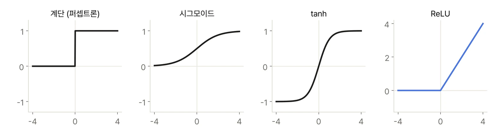
Four common activation functions. The step function jumps abruptly from 0 to 1 at 0, the sigmoid changes smoothly between 0 and 1, tanh changes between −1 and 1, and ReLU outputs 0 for negative inputs and passes positive inputs through unchanged

Function	Formula	Characteristics
Step	1 if $z > 0$	The perceptron. Its gradient is 0 almost everywhere, so it cannot be trained with gradient descent
Sigmoid	$\frac{1}{1 + e^{-z}}$	A smooth step from 0 to 1. Can be interpreted like a probability. When $z$ is large, the gradient approaches 0
tanh	$\frac{e^z - e^{-z}}{e^z + e^{-z}}$	−1 to 1. Its output mean is near 0, so it tends to train better than the sigmoid
ReLU	$\max(0, z)$	Cheapest to compute, and its gradient on the positive side is always 1. The most widely used today

Why the step function is not used for training matters. Gradient descent in the next section moves by following "how much the output changes when a weight changes a little (the gradient)," but the step function is flat almost everywhere, so its gradient is 0. That is why smooth functions (sigmoid, tanh) came into use, and today ReLU has become the standard.

6. Putting a number on how wrong we are: the loss function

To learn, we first need to express "how wrong we are right now" as a single number. This is the loss.

In classification, the last layer outputs a score for each class, and softmax turns those scores into probabilities. It applies the exponential function and then divides so that the sum is 1.

p_k = \frac{e^{s_k}}{\sum_j e^{s_j}}

For example, if the scores for three classes are $(2.0,\ 1.0,\ 0.1)$ , the probabilities are as follows.

Class	Score $s$	$e^{s}$	Probability $p$
0	2.0	7.389	0.659
1	1.0	2.718	0.242
2	0.1	1.105	0.099

The order of the scores is preserved, and the gaps widen. For the loss we use cross-entropy: $-\log$ of the probability assigned to the correct class.

L = -\log p_{\text{correct}}

If the correct answer is class 0, $L = -\log 0.659 = 0.42$ . The correct answer got a high probability, so the loss is small.
If the correct answer is class 2, $L = -\log 0.099 = 2.32$ . The correct answer got a low probability, so the loss is large.
If the probability of the correct answer is 1, $L = 0$ ; as it approaches 0, $L$ grows without bound.

With multiple samples, we use the average of the per-sample losses. Now the goal of learning is clear: find the weights that make this number as small as possible.

7. How to reduce the loss: gradient descent

Let's start with a very simple case that has only one weight. If the loss is $L(w) = (w - 3)^2$ , it is smallest at $w = 3$ . But suppose the computer does not know this answer and descends by looking only at the gradient at its current position.

The gradient is $L'(w) = 2(w - 3)$ . At $w = 0$ the gradient is $-6$ . Being negative means "moving right decreases the loss."
So we move a little in the opposite direction of the gradient. The number that sets the size of each step is the learning rate $\eta$ .

w \leftarrow w - \eta\, L'(w)

Computing just three steps by hand with $\eta = 0.1$ looks like this.

Iteration	$w$	Gradient $2(w-3)$	Next $w = w - 0.1 \times \text{gradient}$
0	0	−6	0.6
1	0.6	−4.8	1.08
2	1.08	−3.84	1.464

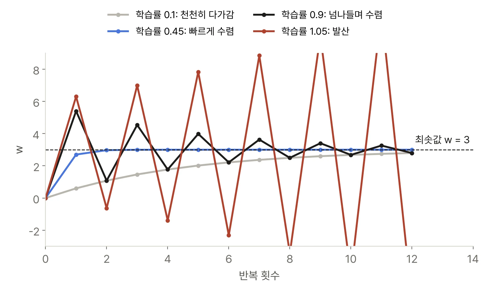
As we approach the minimum, the gradient shrinks and the steps naturally get smaller too. But change the learning rate and the motion becomes completely different.

Gradient descent under different learning rates. 0.1 approaches 3 slowly, 0.45 arrives almost at 3 in two steps, 0.9 converges while bouncing back and forth across 3, and 1.05 diverges as the bounces grow wider

Learning rate	$w$ over the first few steps	Result
0.1	0 → 0.6 → 1.08 → 1.46 → …	Safe but slow
0.45	0 → 2.7 → 2.97 → 3.00	Converges quickly
0.9	0 → 5.4 → 1.08 → 4.54 → …	Bounces across the minimum, then slowly converges
1.05	0 → 6.3 → −0.63 → 6.99 → …	The bounces grow wider and it diverges

For this function, if the learning rate is greater than 1, a single step overshoots the minimum and lands even farther away on the other side. The loss landscape of a real neural network is a bumpy mountain range over millions of weights, but the principle is the same: compute the gradient with respect to every weight, and repeatedly move a little in the opposite direction. This one graph also captures why choosing the learning rate is hard.

Mini-batches and epochs

If there are 60,000 images, computing the loss over all 60,000 for every single step is too slow. So we usually split the data into small groups (mini-batches, e.g. 64 images), estimate the gradient from the average loss of one batch, and take one step at a time (stochastic gradient descent, SGD). Going through the entire dataset once is called an epoch. Looking at 60,000 images 64 at a time takes about 938 steps per epoch.

8. Summary

A neuron is an activation function applied to the weighted sum $z = \sum w_i x_i + b$ . Just changing the weights gives different computations such as AND and OR.
A single neuron only solves problems separable by one straight line. In practice, XOR remained unsolved for all 20 epochs.
Stacking layers lets earlier layers turn the problem into an easier representation, so XOR is solved too. However, there must be a nonlinear activation function between layers.
Learning means defining a loss (softmax + cross-entropy for classification) and reducing it with gradient descent. If the learning rate is too large, training diverges.

Next post: Gradient descent needs the gradient of every weight. If there are 100,000 weights, how do we compute all those gradients at once? In Part 2, we follow backpropagation, which solves this problem with the chain rule, through a numeric example, then implement it ourselves in NumPy and train it on handwritten digits (MNIST).

Practice code: Every number in this post (perceptron training, the XOR network, the softmax example, gradient descent) was computed directly with NumPy. The perceptron started from small random values with a fixed seed.

References

F. Rosenblatt, "The Perceptron: A Probabilistic Model for Information Storage and Organization in the Brain", Psychological Review 65(6), 1958.
M. Minsky, S. Papert, Perceptrons: An Introduction to Computational Geometry, MIT Press, 1969.
I. Goodfellow, Y. Bengio, A. Courville, Deep Learning, Chapter 4 (Numerical Computation and gradient descent), Chapter 6 (Deep Feedforward Networks), MIT Press, 2016.
M. Nielsen, Neural Networks and Deep Learning, Chapter 1.