Chapter 2: Pipelining Overview
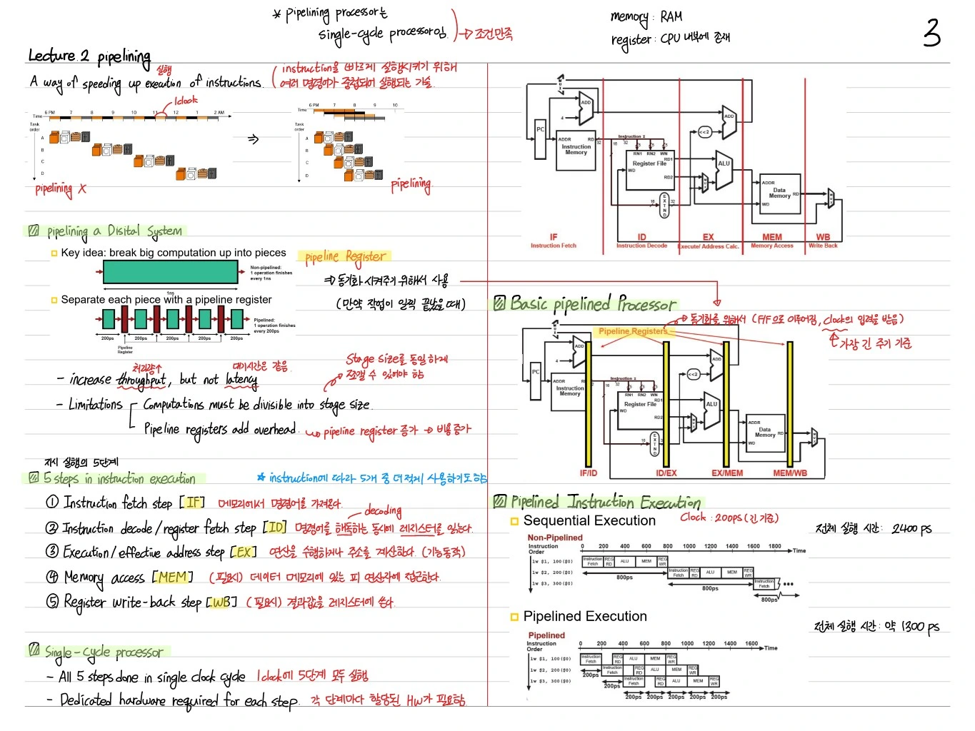
Pipelining is a technique that raises execution speed, not the number of instructions. It splits the processing of one instruction into several stages and runs each stage independently in parallel to increase throughput.
Pipelining in Ordered System
The core idea of pipelining: break the work into stages, isolate each stage with a pipeline register, so that different stages of different instructions run at the same time.
- Advance physical, but not latency
- Limitation: the latency of a single task does not go down
- The pipeline stage time is set by the slowest stage (the slowest stage determines the overall clock period)
5-Stage MIPS Pipeline
The MIPS pipeline usually has 5 stages.
- IF (Instruction Fetch) — read the instruction from memory
- ID (Instruction Decode + Register read) — decode and read registers
- EX (Execute) — ALU operation
- MEM (Memory access) — memory access for load/store
- WB (Write Back) — write the result to a register
Sequential vs Pipelined Performance
When executing the same instructions:
- Sequential execution: each instruction finishes every stage before the next one starts (e.g., 8 ns × 3 instructions)
- Pipelined execution: stages overlap → total time shrinks to 2 ns × (3 + 4) = about 14 ns
So with more instructions, throughput ideally increases by the number of stages.
Hazards — The Enemy of the Pipeline
Three kinds of hazards keep a pipeline from running ideally:
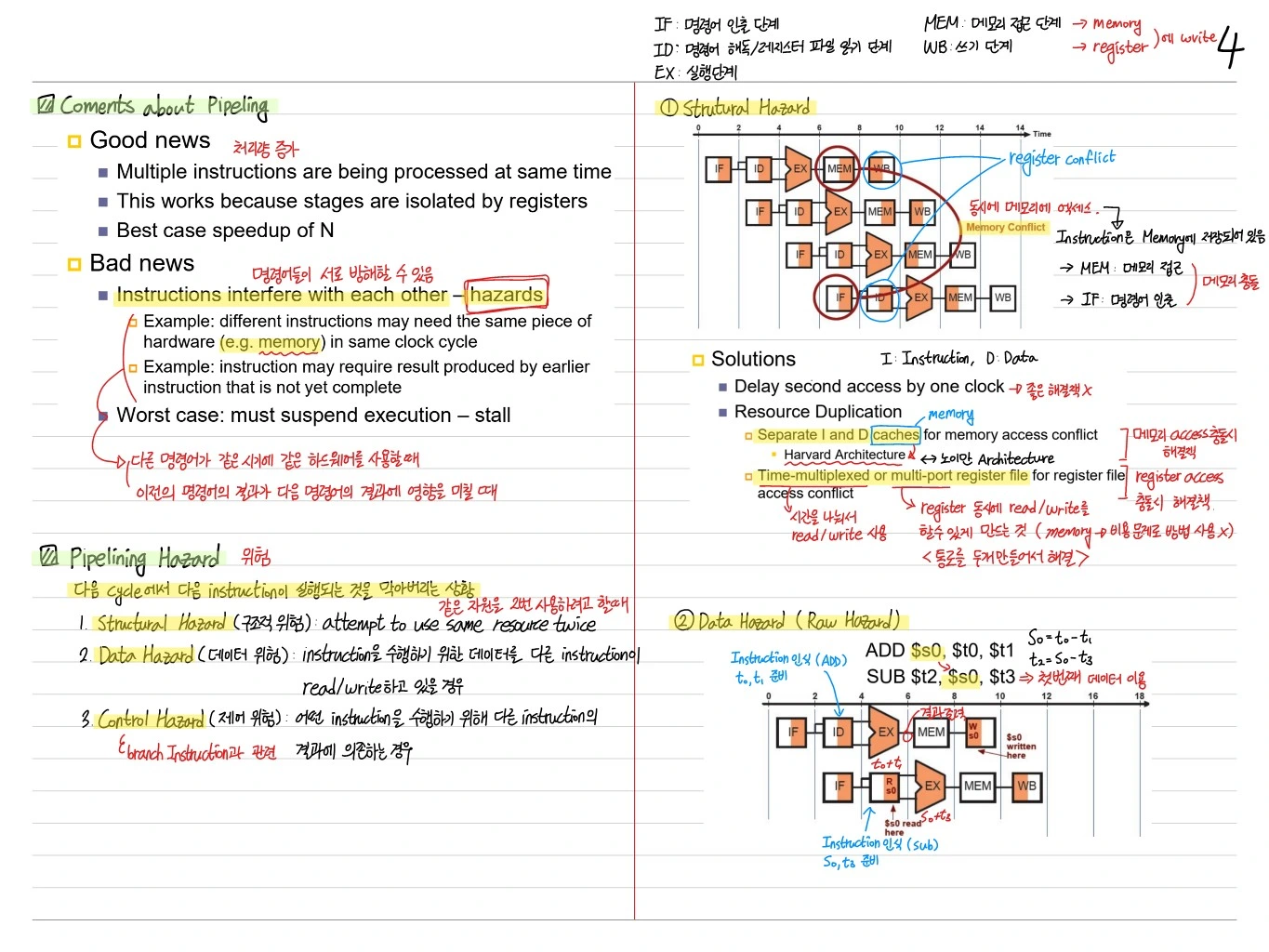
1. Structural Hazard
Multiple instructions are being processed at same time.
Example: a conflict when IF and MEM use a single memory at the same time. → Solutions:
- Replicate resources (separate I-cache / D-cache)
- Isolate each stage with pipeline registers
2. Data Hazard
When the next instruction needs the result of a previous instruction.
Example:
add r1, r2, r3    # writes a value to r1
sub r4, r1, r5    # immediately reads r1 → r1 not yet written back
If a later instruction reads before the previous instruction reaches WB, it gets the wrong value. Worst case: suspend execution — stall.
Solutions
- Delay second access — stop until the previous instruction's result arrives (stall / bubble)
- Resource Duplication
- Forwarding (Bypassing): pass the ALU result straight to the EX input without waiting for WB. A direct connection from the pipeline register to the next stage.
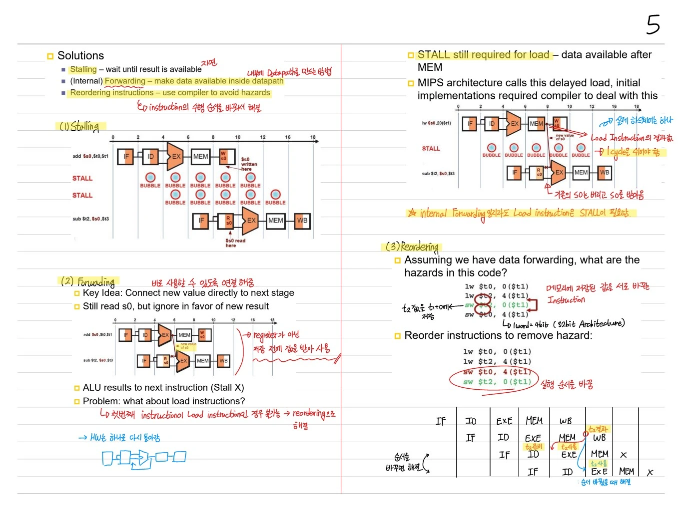
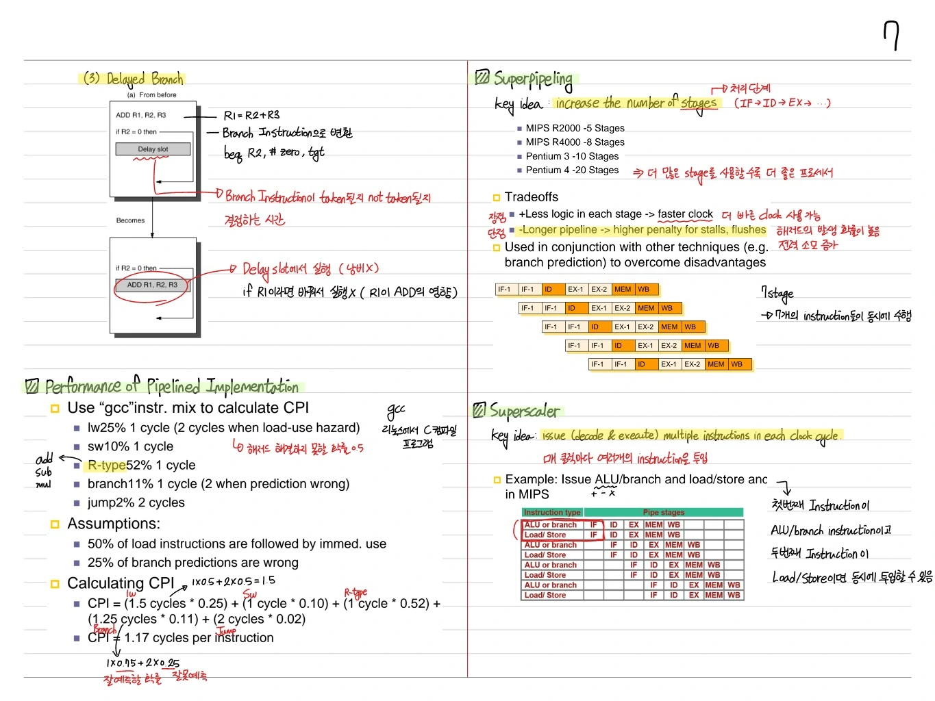
Load-Use Data Hazard
A case forwarding cannot fix: using a value right after loading it. The loaded value comes out at the end of the MEM stage, so it cannot reach the next instruction before its EX → a 1-cycle stall is required.
MIPS architecture calls this delayed load, initial implementations required compiler to deal with this.
Stall / Bubble
- Key idea: Connect new value directly to next stage
- Still need to stall for stalls → handles the load-use case for load instructions
- ALU results to next instruction (no stall)
- Problem: what about load instructions? → stall the next instruction + forward
3. Control Hazard (Branch Hazard)
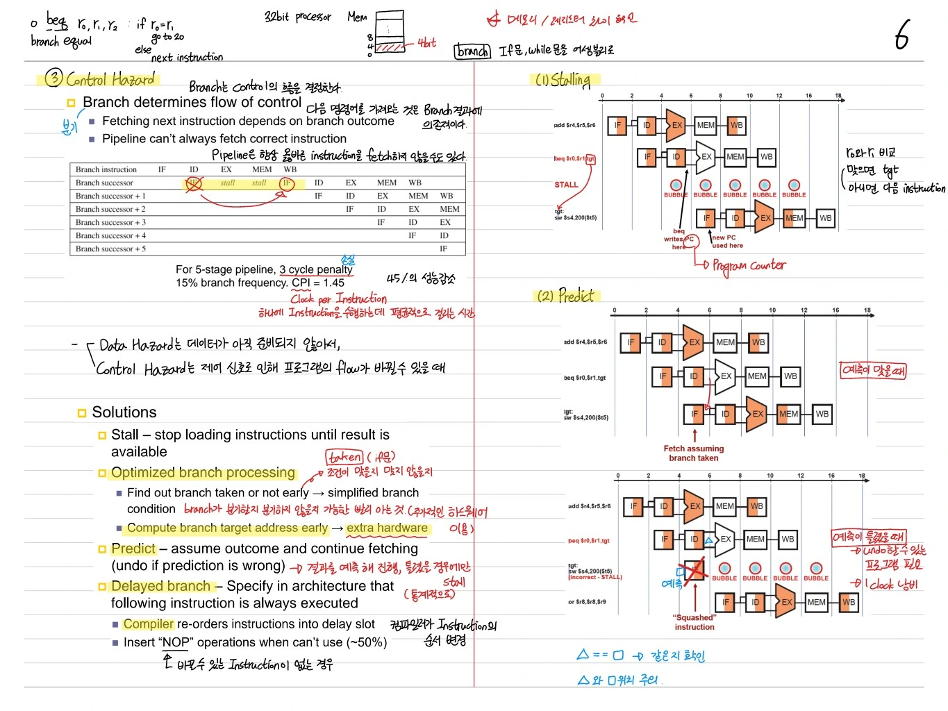
Branch determines flow of control. If later instructions are fetched before the branch outcome is resolved, the wrong instructions may execute.
- Pipeline can't always fetch correct instruction — the PC must be decided in the fetch stage, but the branch is not resolved before EX
- Branch penalty for a 5-stage pipeline with 10% branches:
→ 10% branches × 3-cycle stall = 15% branch impact → 20% performance loss for MIPS
Solutions
- Stall — simple, but loading instructions until result is available
- Compromise branch processing — simplified branch condition
- Prediction — assume outcome and continue fetching (predict not-taken → flush if wrong)
- Delayed branch — compiler schedules a useful instruction into the delay slot (MIPS)
- Compile re-orders instructions into delay slot. Insert
nop(no operation) instructions when can't reorder.
Performance of a Pipelined Implementation
Worked CPI Example
- Use "gcc" instruction mix to calculate CPI
- IW = 25% (2 cycles when load-use happen)
- SW = 10% (1 cycle)
- R-type = 52%
- Branch = 11% (1 cycle delayed branches)
- Jump = 2% (1 cycle)
Assumption: 50% of load instructions are followed by immed. use.
→ Thanks to pipelining, the effect is 1.17 cycles per instruction.
Superpipelining
Key idea: Increase the number of stages. Example: Pentium 4 → 20 stages.
- Advantages: Faster clock (each stage is short)
- Disadvantages: Longer pipeline → higher branch penalty, more flushes
- Used in conjunction with other techniques to overcome disadvantages (branch prediction)
Superscalar
Key idea: Issue (and execute) multiple instructions in each clock cycle.
Example: Issue ALU/branch and load/store at MIPS:
| ALU / branch | Load / Store |
|---|---|
| nop | lw s1) |
| add s1, $s0 | sw s1) |
| nop | ... |
→ Multiple instructions are issued at the same time. But scheduling to respect dependencies gets complex.
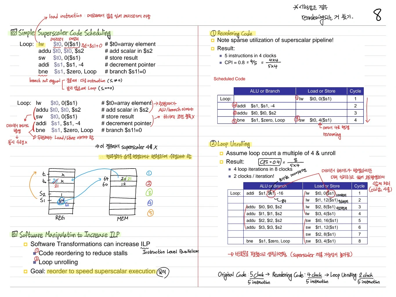
Software Manipulation to Increase ILP
Simple Superscalar Code Scheduling
Loop:
  lw   $t0, 0($s1)   # $t0 = array element
  addu $t0, $t0, $s2 # add scalar in $s2
  sw   $t0, 0($s1)   # store result
  addi $s1, $s1, -4  # decrement pointer
  bne  $s1, $zero, Loop  # branch $s1 != 0
Reordering — Moving Independent Instructions
Note: Update value of $t0 will not be available for next iteration → placing dependent instructions farther apart avoids stalls.
Loop Unrolling
Assume loop count is multiple of 4, & unroll 4 loop iterations in 4 cycles.
Loop:
  lw $t0, 0($s1)   lw $t1, -4($s1)
  lw $t2, -8($s1)  lw $t3, -12($s1)
  addu $t0, $t0, $s2  addu $t1, $t1, $s2
  ...
→ On a superscalar machine, 4 × IPC = 4 cycles per 4 iterations (ideal)
Dynamic Pipeline Scheduling
A technique that dynamically changes the order of instructions while the program runs. Done by the hardware, not the compiler.
Out-of-order Execute, In-order Commit
Instruction Fetch & Decode unit (In-order issue)
         │
   ┌─────┼─────┬─────┬─────┐
   ▼     ▼     ▼     ▼
 Reservation stations (× N)
   │     │     │     │
   ▼     ▼     ▼     ▼
Integer  Integer  Floating point  Load/Store
   │     │     │     │
   ▼     ▼     ▼     ▼
Commit unit (In-order commit)- Example: Power PC 604, Pentium Pro, Alpha 21264, MIPS R10000
- Instructions are sorted into reservation stations by type (not by compile order)
- Out-of-order execute → whatever is ready runs first
- Commit happens in order
Overcomes Key Performance Limitations
- Structural hazard → Replicate pipelines
- Data hazard → Execute instructions out of program order, Rename registers as needed
- Control hazard → Execute instructions speculatively across branches (speculative execution)
Instructions that are hard to process can be skipped for now → fewer stalls.
Dynamic Branch Prediction
Predicting branches while the program runs (↔ static prediction, done before execution).
One-bit Prediction Scheme
- For each branch, store in one bit whether it was taken or not taken last time, and predict from that
- Example: a loop like
for (i=0; i<10000; i++)is Good (mostly taken) - Problem: Loop case (mispredicts on the last iteration)
Give each branch a register that stores whether it was taken or not taken last time, and predict from it.
Two-bit Prediction Scheme
State machine: instead of two states, predict taken / not-taken, there are 4 states (strong taken, weak taken, weak not-taken, strong not-taken).
- One misprediction does not immediately flip the prediction → high accuracy even in the loop case
- Predicts both the inner and outer for loops well in nested loops
for (i=0; i<10000; i++)       ← outer
  for (j=0; j<10000; j++)     ← inner (mostly taken)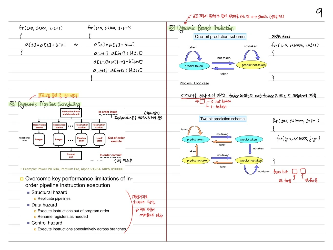
Summary
| Technique | Purpose | Typical example |
|---|---|---|
| Pipelining | Throughput ↑ | 5-stage MIPS |
| Forwarding | Minimize data hazards | EX → EX bypass |
| Delayed branch | Mitigate control hazards | MIPS 1-cycle delay slot |
| Superscalar | IPC ↑ | Pentium Pro |
| Superpipelining | Clock ↑ | Pentium 4 (20 stages) |
| Out-of-order | Hardware scheduling | R10000, Alpha 21264 |
| Branch Prediction (2-bit) | Branch accuracy ↑ | Standard in modern CPUs |
Pipelining and its variants are the foundation of hardware parallelism, and they underpin everything that follows: the cache hierarchy, virtual memory, and multi-core.